

2.6 Dynamics of Defects
37
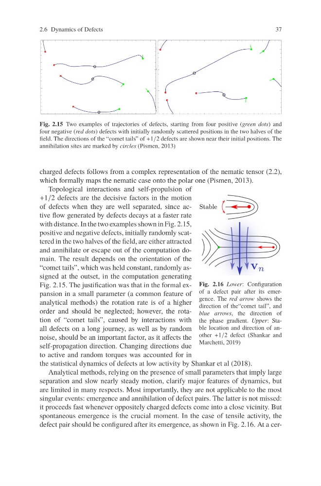
Fig. 2.15 Two examples of trajectories of defects, starting from four positive (green dots) and
four negative (red dots) defects with initially randomly scattered positions in the two halves of the
field. The directions of the “comet tails” of +1/2 defects are shown near their initial positions. The
annihilation sites are marked by circles (Pismen, 2013)
charged defects follows from a complex representation of the nematic tensor (2.2),
which formally maps the nematic case onto the polar one (Pismen, 2013).
Fig. 2.16 Lower: Configuration
of a defect pair after its emergence. The red arrow shows the
direction of the“comet tail”, and
blue arrows, the direction of
the phase gradient. Upper: Stable location and direction of another +1/2 defect (Shankar and
Marchetti, 2019)
Topological interactions and self-propulsion of
+1/2 defects are the decisive factors in the motion
of defects when they are well separated, since active flow generated by defects decays at a faster rate
with distance. In the two examples shown in Fig. 2.15,
positive and negative defects, initially randomly scattered in the two halves of the field, are either attracted
and annihilate or escape out of the computation domain. The result depends on the orientation of the
“comet tails”, which was held constant, randomly assigned at the outset, in the computation generating
Fig. 2.15. The justification was that in the formal expansion in a small parameter (a common feature of
analytical methods) the rotation rate is of a higher
order and should be neglected; however, the rotation of “comet tails”, caused by interactions with
all defects on a long journey, as well as by random
noise, should be an important factor, as it affects the
self-propagation direction. Changing directions due
to active and random torques was accounted for in
the statistical dynamics of defects at low activity by Shankar et al (2018).
Analytical methods, relying on the presence of small parameters that imply large
separation and slow nearly steady motion, clarify major features of dynamics, but
are limited in many respects. Most importantly, they are not applicable to the most
singular events: emergence and annihilation of defect pairs. The latter is not missed:
it proceeds fast whenever oppositely charged defects come into a close vicinity. But
spontaneous emergence is the crucial moment. In the case of tensile activity, the
defect pair should be configured after its emergence, as shown in Fig. 2.16. At a cer-
37
Fig. 2.15 Two examples of trajectories of defects, starting from four positive (green dots) and
four negative (red dots) defects with initially randomly scattered positions in the two halves of the
field. The directions of the “comet tails” of +1/2 defects are shown near their initial positions. The
annihilation sites are marked by circles (Pismen, 2013)
charged defects follows from a complex representation of the nematic tensor (2.2),
which formally maps the nematic case onto the polar one (Pismen, 2013).
Fig. 2.16 Lower: Configuration
of a defect pair after its emergence. The red arrow shows the
direction of the“comet tail”, and
blue arrows, the direction of
the phase gradient. Upper: Stable location and direction of another +1/2 defect (Shankar and
Marchetti, 2019)
Topological interactions and self-propulsion of
+1/2 defects are the decisive factors in the motion
of defects when they are well separated, since active flow generated by defects decays at a faster rate
with distance. In the two examples shown in Fig. 2.15,
positive and negative defects, initially randomly scattered in the two halves of the field, are either attracted
and annihilate or escape out of the computation domain. The result depends on the orientation of the
“comet tails”, which was held constant, randomly assigned at the outset, in the computation generating
Fig. 2.15. The justification was that in the formal expansion in a small parameter (a common feature of
analytical methods) the rotation rate is of a higher
order and should be neglected; however, the rotation of “comet tails”, caused by interactions with
all defects on a long journey, as well as by random
noise, should be an important factor, as it affects the
self-propagation direction. Changing directions due
to active and random torques was accounted for in
the statistical dynamics of defects at low activity by Shankar et al (2018).
Analytical methods, relying on the presence of small parameters that imply large
separation and slow nearly steady motion, clarify major features of dynamics, but
are limited in many respects. Most importantly, they are not applicable to the most
singular events: emergence and annihilation of defect pairs. The latter is not missed:
it proceeds fast whenever oppositely charged defects come into a close vicinity. But
spontaneous emergence is the crucial moment. In the case of tensile activity, the
defect pair should be configured after its emergence, as shown in Fig. 2.16. At a cer-