

142
7 Live Tissues
A natural and economical way of simulating rearrangements of structured layers
is the vertex model, widely used in the description of all kinds of structures composed of nearly-uniform domains of polygonal or polyhedral shape (Stavans, 1993).
Natural planar tilings are hexagonal. Hexagonal patterns arise in symmetry-breaking
bifurcations due to the resonance interaction of a triplet of modes. This causes, for
example, common patterns of Bénard convection, driven either by gravity or surface
tension gradients, shown in Fig. 7.1a. But a still deeper reason lies in topology. The
generic number of edges joining a vertex in a random tiling is three. Even in such an
artificial tiling as the map of the USA there is a single “four-corners” point. If each
of N cells in an infinite tiling has Q edges, the number of vertices is V =
1
3 QN and
the number of edges is E =
1
2 QN. These numbers are related by the classical Euler
theorem: N + V − E = 1. Neglecting unity in an infinite tiling, this yields Q = 6, i.e.,
a hexagonal pattern.
Fig. 7.2 Example of a
Voronoi tessellation (CC)
Cellular patterns in epithelial layers, like the one in
Fig. 7.1b, are not as neat, but the average number of neighbors comes very close to six anyway. Miklius and Hilgenfeldt (2011) compiled thorough statistics of different samples and detected a minuscular shift, easily attributed to
the inability to resolve some edges separating neighboring cells, leading to apparent four-fold junctions between
cells, and the finite size of the experimental samples.
Even rather regular patterns, like the one in Fig. 7.1a,
contain defects. The generic topological defect in a hexagonal tiling is the penta-hepta defect, a pair of cells with five
and seven neighbors, accentuated by colors in Fig. 7.1a. A
non-generic defect, also present in this picture, is a rosette,
which is easily resolved by inserting a small cell in its center.
A simulation may be initiated by a tiling generated by Voronoi tessellation. A
random set of generating points is chosen, and cell borders are drawn normally to
the lines connecting nearby points as far as intersections with other lines. Formally,
each tile should contain points closer to the respective generating point than to other
points from the generating set. This creates a very irregular pattern, like the one
shown in Fig. 7.2. In some simulations, positions of generating points, interpreted
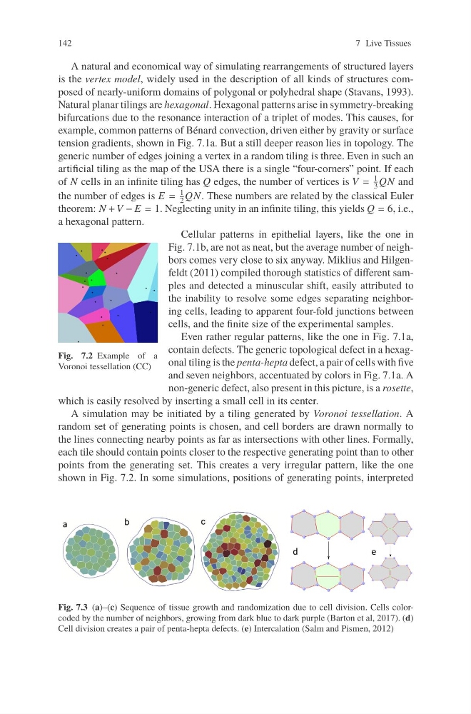
Fig. 7.3 (a)–(c) Sequence of tissue growth and randomization due to cell division. Cells colorcoded by the number of neighbors, growing from dark blue to dark purple (Barton et al, 2017). (d)
Cell division creates a pair of penta-hepta defects. (e) Intercalation (Salm and Pismen, 2012)
7 Live Tissues
A natural and economical way of simulating rearrangements of structured layers
is the vertex model, widely used in the description of all kinds of structures composed of nearly-uniform domains of polygonal or polyhedral shape (Stavans, 1993).
Natural planar tilings are hexagonal. Hexagonal patterns arise in symmetry-breaking
bifurcations due to the resonance interaction of a triplet of modes. This causes, for
example, common patterns of Bénard convection, driven either by gravity or surface
tension gradients, shown in Fig. 7.1a. But a still deeper reason lies in topology. The
generic number of edges joining a vertex in a random tiling is three. Even in such an
artificial tiling as the map of the USA there is a single “four-corners” point. If each
of N cells in an infinite tiling has Q edges, the number of vertices is V =
1
3 QN and
the number of edges is E =
1
2 QN. These numbers are related by the classical Euler
theorem: N + V − E = 1. Neglecting unity in an infinite tiling, this yields Q = 6, i.e.,
a hexagonal pattern.
Fig. 7.2 Example of a
Voronoi tessellation (CC)
Cellular patterns in epithelial layers, like the one in
Fig. 7.1b, are not as neat, but the average number of neighbors comes very close to six anyway. Miklius and Hilgenfeldt (2011) compiled thorough statistics of different samples and detected a minuscular shift, easily attributed to
the inability to resolve some edges separating neighboring cells, leading to apparent four-fold junctions between
cells, and the finite size of the experimental samples.
Even rather regular patterns, like the one in Fig. 7.1a,
contain defects. The generic topological defect in a hexagonal tiling is the penta-hepta defect, a pair of cells with five
and seven neighbors, accentuated by colors in Fig. 7.1a. A
non-generic defect, also present in this picture, is a rosette,
which is easily resolved by inserting a small cell in its center.
A simulation may be initiated by a tiling generated by Voronoi tessellation. A
random set of generating points is chosen, and cell borders are drawn normally to
the lines connecting nearby points as far as intersections with other lines. Formally,
each tile should contain points closer to the respective generating point than to other
points from the generating set. This creates a very irregular pattern, like the one
shown in Fig. 7.2. In some simulations, positions of generating points, interpreted
Fig. 7.3 (a)–(c) Sequence of tissue growth and randomization due to cell division. Cells colorcoded by the number of neighbors, growing from dark blue to dark purple (Barton et al, 2017). (d)
Cell division creates a pair of penta-hepta defects. (e) Intercalation (Salm and Pismen, 2012)