

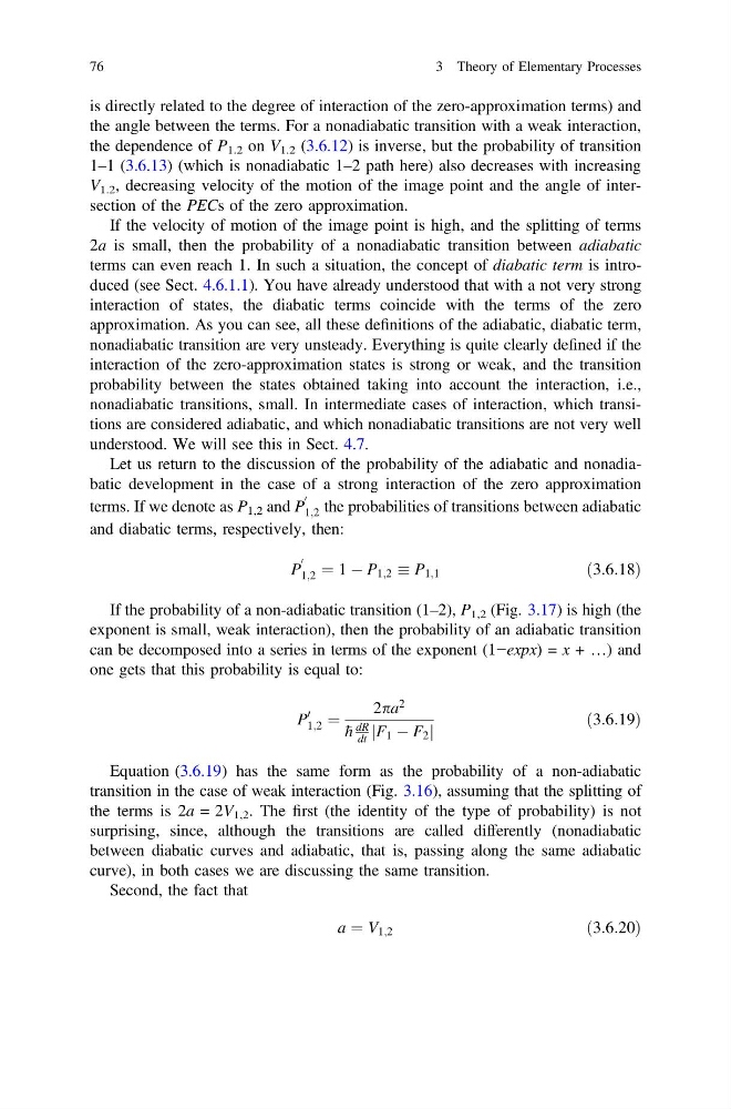
is directly related to the degree of interaction of the zero-approximation terms) and
the angle between the terms. For a nonadiabatic transition with a weak interaction,
the dependence of P 1.2 on V 1.2 (3.6.12) is inverse, but the probability of transition
1–1 (3.6.13) (which is nonadiabatic 1–2 path here) also decreases with increasing
V 1.2 , decreasing velocity of the motion of the image point and the angle of intersection of the PECs of the zero approximation.
If the velocity of motion of the image point is high, and the splitting of terms
2a is small, then the probability of a nonadiabatic transition between adiabatic
terms can even reach 1. In such a situation, the concept of diabatic term is introduced (see Sect. 4.6.1.1). You have already understood that with a not very strong
interaction of states, the diabatic terms coincide with the terms of the zero
approximation. As you can see, all these definitions of the adiabatic, diabatic term,
nonadiabatic transition are very unsteady. Everything is quite clearly defined if the
interaction of the zero-approximation states is strong or weak, and the transition
probability between the states obtained taking into account the interaction, i.e.,
nonadiabatic transitions, small. In intermediate cases of interaction, which transitions are considered adiabatic, and which nonadiabatic transitions are not very well
understood. We will see this in Sect. 4.7.
Let us return to the discussion of the probability of the adiabatic and nonadiabatic development in the case of a strong interaction of the zero approximation
terms. If we denote as P 1,2 and P
0
1;2 the probabilities of transitions between adiabatic
and diabatic terms, respectively, then:
P
0
1;2 ¼ 1 À P 1;2 P 1;1
ð3:6:18Þ
If the probability of a non-adiabatic transition (1–2), P 1,2 (Fig. 3.17) is high (the
exponent is small, weak interaction), then the probability of an adiabatic transition
can be decomposed into a series in terms of the exponent (1−expx) = x + …) and
one gets that this probability is equal to:
P
0
1;2 ¼
2pa
2
h
dR
dt F 1 À F 2
j
j
ð3:6:19Þ
Equation (3.6.19) has the same form as the probability of a non-adiabatic
transition in the case of weak interaction (Fig. 3.16), assuming that the splitting of
the terms is 2a = 2V 1,2 . The first (the identity of the type of probability) is not
surprising, since, although the transitions are called differently (nonadiabatic
between diabatic curves and adiabatic, that is, passing along the same adiabatic
curve), in both cases we are discussing the same transition.
Second, the fact that
a ¼ V 1;2
ð3:6:20Þ
76
3 Theory of Elementary Processes
the angle between the terms. For a nonadiabatic transition with a weak interaction,
the dependence of P 1.2 on V 1.2 (3.6.12) is inverse, but the probability of transition
1–1 (3.6.13) (which is nonadiabatic 1–2 path here) also decreases with increasing
V 1.2 , decreasing velocity of the motion of the image point and the angle of intersection of the PECs of the zero approximation.
If the velocity of motion of the image point is high, and the splitting of terms
2a is small, then the probability of a nonadiabatic transition between adiabatic
terms can even reach 1. In such a situation, the concept of diabatic term is introduced (see Sect. 4.6.1.1). You have already understood that with a not very strong
interaction of states, the diabatic terms coincide with the terms of the zero
approximation. As you can see, all these definitions of the adiabatic, diabatic term,
nonadiabatic transition are very unsteady. Everything is quite clearly defined if the
interaction of the zero-approximation states is strong or weak, and the transition
probability between the states obtained taking into account the interaction, i.e.,
nonadiabatic transitions, small. In intermediate cases of interaction, which transitions are considered adiabatic, and which nonadiabatic transitions are not very well
understood. We will see this in Sect. 4.7.
Let us return to the discussion of the probability of the adiabatic and nonadiabatic development in the case of a strong interaction of the zero approximation
terms. If we denote as P 1,2 and P
0
1;2 the probabilities of transitions between adiabatic
and diabatic terms, respectively, then:
P
0
1;2 ¼ 1 À P 1;2 P 1;1
ð3:6:18Þ
If the probability of a non-adiabatic transition (1–2), P 1,2 (Fig. 3.17) is high (the
exponent is small, weak interaction), then the probability of an adiabatic transition
can be decomposed into a series in terms of the exponent (1−expx) = x + …) and
one gets that this probability is equal to:
P
0
1;2 ¼
2pa
2
h
dR
dt F 1 À F 2
j
j
ð3:6:19Þ
Equation (3.6.19) has the same form as the probability of a non-adiabatic
transition in the case of weak interaction (Fig. 3.16), assuming that the splitting of
the terms is 2a = 2V 1,2 . The first (the identity of the type of probability) is not
surprising, since, although the transitions are called differently (nonadiabatic
between diabatic curves and adiabatic, that is, passing along the same adiabatic
curve), in both cases we are discussing the same transition.
Second, the fact that
a ¼ V 1;2
ð3:6:20Þ
76
3 Theory of Elementary Processes