

surface in 5-dimensional space. But, if we ‘freeze’ two bending coordinate, for
example, if we make the angle c equal to 0, then we get a two-dimensional surface in
three-dimensional space. This is a completely ‘presentable’ thing.
It can be ‘decorated’ using lines corresponding to constant potential energy,
equipotential lines, and it is quite tangible to imagine the relative motion of atoms
as the motion of a point of mass l, called the image (representative) point of this
potential well. And not only to present but also to calculate.
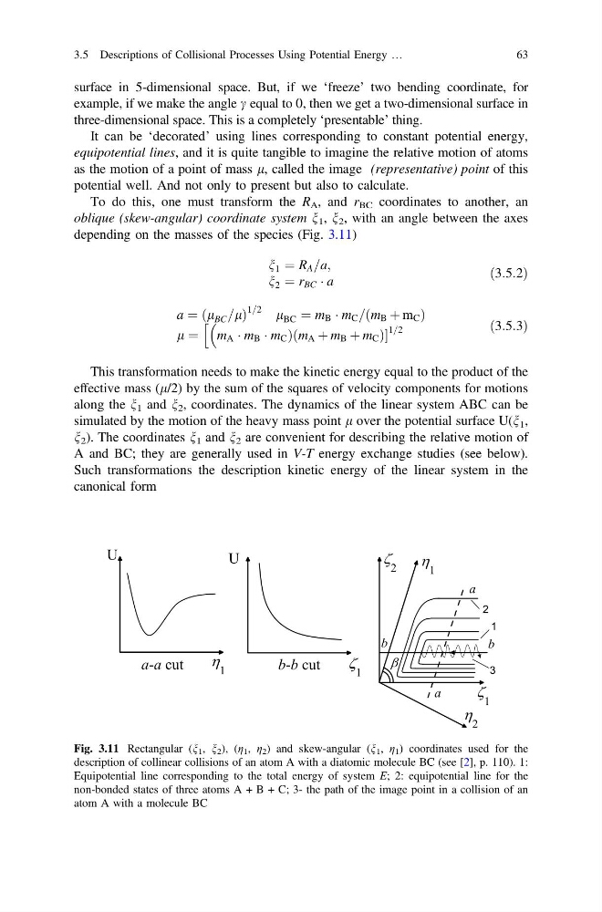
To do this, one must transform the R A , and r BC coordinates to another, an
oblique (skew-angular) coordinate system n 1 , n 2 , with an angle between the axes
depending on the masses of the species (Fig. 3.11)
n 1 ¼ R A =a;
n 2 ¼ r BC Á a
ð3:5:2Þ
a ¼ l BC =l
ð
Þ
1=2 l BC ¼ m B Á m C = m B þ m C
ð
Þ
l ¼ m A Á m B Á m C Þðm A þ m B þ m C Þ
1=2
h
ð3:5:3Þ
This transformation needs to make the kinetic energy equal to the product of the
effective mass (l/2) by the sum of the squares of velocity components for motions
along the n 1 and n 2 , coordinates. The dynamics of the linear system ABC can be
simulated by the motion of the heavy mass point l over the potential surface U(n 1 ,
n 2 ). The coordinates n 1 and n 2 are convenient for describing the relative motion of
A and BC; they are generally used in V-T energy exchange studies (see below).
Such transformations the description kinetic energy of the linear system in the
canonical form
Fig. 3.11 Rectangular (n 1 , n 2 ), (η 1 , η 2 ) and skew-angular (n 1 , η 1 ) coordinates used for the
description of collinear collisions of an atom A with a diatomic molecule BC (see [2], p. 110). 1:
Equipotential line corresponding to the total energy of system E; 2: equipotential line for the
non-bonded states of three atoms A + B + C; 3- the path of the image point in a collision of an
atom A with a molecule BC
3.5 Descriptions of Collisional Processes Using Potential Energy …
63
example, if we make the angle c equal to 0, then we get a two-dimensional surface in
three-dimensional space. This is a completely ‘presentable’ thing.
It can be ‘decorated’ using lines corresponding to constant potential energy,
equipotential lines, and it is quite tangible to imagine the relative motion of atoms
as the motion of a point of mass l, called the image (representative) point of this
potential well. And not only to present but also to calculate.
To do this, one must transform the R A , and r BC coordinates to another, an
oblique (skew-angular) coordinate system n 1 , n 2 , with an angle between the axes
depending on the masses of the species (Fig. 3.11)
n 1 ¼ R A =a;
n 2 ¼ r BC Á a
ð3:5:2Þ
a ¼ l BC =l
ð
Þ
1=2 l BC ¼ m B Á m C = m B þ m C
ð
Þ
l ¼ m A Á m B Á m C Þðm A þ m B þ m C Þ
1=2
h
ð3:5:3Þ
This transformation needs to make the kinetic energy equal to the product of the
effective mass (l/2) by the sum of the squares of velocity components for motions
along the n 1 and n 2 , coordinates. The dynamics of the linear system ABC can be
simulated by the motion of the heavy mass point l over the potential surface U(n 1 ,
n 2 ). The coordinates n 1 and n 2 are convenient for describing the relative motion of
A and BC; they are generally used in V-T energy exchange studies (see below).
Such transformations the description kinetic energy of the linear system in the
canonical form
Fig. 3.11 Rectangular (n 1 , n 2 ), (η 1 , η 2 ) and skew-angular (n 1 , η 1 ) coordinates used for the
description of collinear collisions of an atom A with a diatomic molecule BC (see [2], p. 110). 1:
Equipotential line corresponding to the total energy of system E; 2: equipotential line for the
non-bonded states of three atoms A + B + C; 3- the path of the image point in a collision of an
atom A with a molecule BC
3.5 Descriptions of Collisional Processes Using Potential Energy …
63