

resolution; however, it is often possible to estimate matrix elements averaged over
hyperfine components. The coupling of the mentioned above IP states was studied
using simpler methods.
The excitation of the coupled E0
þ
g * c1 u states was performed by the standard
optical–optical double resonance (OODR) E ← B ← X scheme (see Sect. 2.12.1
in [7]). Two pairs of vibrational levels are close enough to find effective hyperfine
coupling in the low-v range: v E = 3 * v c = 1 and v E = 19 * v c = 18. Selection
rules DJ = 0, ± 1, and ± 2 allow to couple different vibrational states at some
rotational quantum numbers (Fig. 4.16).
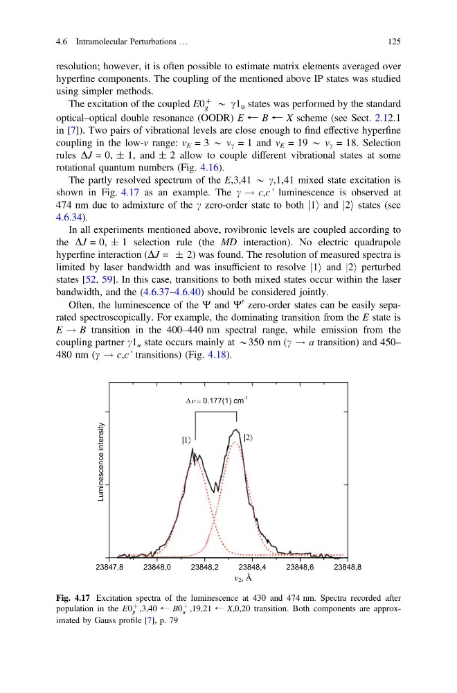
The partly resolved spectrum of the E,3,41 * c,1,41 mixed state excitation is
shown in Fig. 4.17 as an example. The c ! c,c’ luminescence is observed at
474 nm due to admixture of the c zero-order state to both 1
j i and 2
j i states (see
4.6.34).
In all experiments mentioned above, rovibronic levels are coupled according to
the DJ = 0, ± 1 selection rule (the MD interaction). No electric quadrupole
hyperfine interaction (DJ = ± 2) was found. The resolution of measured spectra is
limited by laser bandwidth and was insufficient to resolve 1
j i and 2
j i perturbed
states [52, 59]. In this case, transitions to both mixed states occur within the laser
bandwidth, and the (4.6.37–4.6.40) should be considered jointly.
Often, the luminescence of the W and W
0 zero-order states can be easily separated spectroscopically. For example, the dominating transition from the E state is
E ! B transition in the 400–440 nm spectral range, while emission from the
coupling partner c1 u state occurs mainly at *350 nm (c ! a transition) and 450–
480 nm (c ! c,c’ transitions) (Fig. 4.18).
Fig. 4.17 Excitation spectra of the luminescence at 430 and 474 nm. Spectra recorded after
population in the E0
þ
g ,3,40 ← B0
þ
u ,19,21 ← X,0,20 transition. Both components are approximated by Gauss profile [7], p. 79
4.6 Intramolecular Perturbations …
125
hyperfine components. The coupling of the mentioned above IP states was studied
using simpler methods.
The excitation of the coupled E0
þ
g * c1 u states was performed by the standard
optical–optical double resonance (OODR) E ← B ← X scheme (see Sect. 2.12.1
in [7]). Two pairs of vibrational levels are close enough to find effective hyperfine
coupling in the low-v range: v E = 3 * v c = 1 and v E = 19 * v c = 18. Selection
rules DJ = 0, ± 1, and ± 2 allow to couple different vibrational states at some
rotational quantum numbers (Fig. 4.16).
The partly resolved spectrum of the E,3,41 * c,1,41 mixed state excitation is
shown in Fig. 4.17 as an example. The c ! c,c’ luminescence is observed at
474 nm due to admixture of the c zero-order state to both 1
j i and 2
j i states (see
4.6.34).
In all experiments mentioned above, rovibronic levels are coupled according to
the DJ = 0, ± 1 selection rule (the MD interaction). No electric quadrupole
hyperfine interaction (DJ = ± 2) was found. The resolution of measured spectra is
limited by laser bandwidth and was insufficient to resolve 1
j i and 2
j i perturbed
states [52, 59]. In this case, transitions to both mixed states occur within the laser
bandwidth, and the (4.6.37–4.6.40) should be considered jointly.
Often, the luminescence of the W and W
0 zero-order states can be easily separated spectroscopically. For example, the dominating transition from the E state is
E ! B transition in the 400–440 nm spectral range, while emission from the
coupling partner c1 u state occurs mainly at *350 nm (c ! a transition) and 450–
480 nm (c ! c,c’ transitions) (Fig. 4.18).
Fig. 4.17 Excitation spectra of the luminescence at 430 and 474 nm. Spectra recorded after
population in the E0
þ
g ,3,40 ← B0
þ
u ,19,21 ← X,0,20 transition. Both components are approximated by Gauss profile [7], p. 79
4.6 Intramolecular Perturbations …
125