

1 Introduction to Nonequilibrium Statistical Physics and Its Foundations
31
E
η(t)
R
η(t
)
R
=
2k B T
R
δ(t − t
) ⇒ q Q =
2k B T
R
E
η(t)
RC
η(t
)
RC
=
2k B T
RC 2 δ(t − t
) ⇒ q U =
2k B T
RC 2
(1.114)
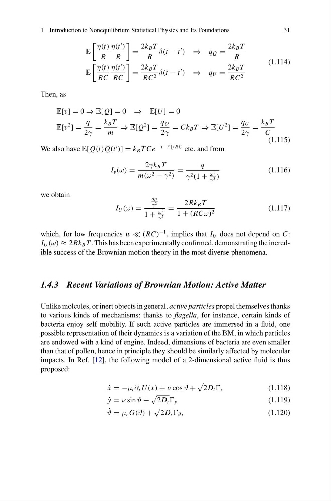
Then, as
E[v] = 0 ⇒ E[Q] = 0 ⇒ E[U ] = 0
E[v
2
] =
q
2γ
=
k B T
m
⇒ E[Q
2
] =
q Q
2γ
= Ck B T ⇒ E[U
2
] =
q U
2γ
=
k B T
C
(1.115)
We also have E[Q(t)Q(t
)] = k B T Ce
−|t−t
|/RC etc. and from
I v (ω) =
2γk B T
m(ω 2 + γ 2 )
=
q
γ 2 (1 +
ω 2
γ 2 )
(1.116)
we obtain
I U (ω) =
q U
γ 2
1 +
ω 2
γ 2
=
2Rk B T
1 + (RCω) 2
(1.117)
which, for low frequencies w (RC)
−1 , implies that I U does not depend on C:
I U (ω) ≈ 2Rk B T . This has been experimentally confirmed, demonstrating the incredible success of the Brownian motion theory in the most diverse phenomena.
1.4.3 Recent Variations of Brownian Motion: Active Matter
Unlike molcules, or inert objects in general, active particles propel themselves thanks
to various kinds of mechanisms: thanks to flagella, for instance, certain kinds of
bacteria enjoy self mobility. If such active particles are immersed in a fluid, one
possible representation of their dynamics is a variation of the BM, in which particles
are endowed with a kind of engine. Indeed, dimensions of bacteria are even smaller
than that of pollen, hence in principle they should be similarly affected by molecular
impacts. In Ref. [12], the following model of a 2-dimensional active fluid is thus
proposed:
˙
x = −μ t ∂ x U (x) + ν cos ϑ +
2D t x
(1.118)
˙
y = ν sin ϑ +
2D t y
(1.119)
˙
ϑ = μ r G(ϑ) +
2D r θ ,
(1.120)
31
E
η(t)
R
η(t
)
R
=
2k B T
R
δ(t − t
) ⇒ q Q =
2k B T
R
E
η(t)
RC
η(t
)
RC
=
2k B T
RC 2 δ(t − t
) ⇒ q U =
2k B T
RC 2
(1.114)
Then, as
E[v] = 0 ⇒ E[Q] = 0 ⇒ E[U ] = 0
E[v
2
] =
q
2γ
=
k B T
m
⇒ E[Q
2
] =
q Q
2γ
= Ck B T ⇒ E[U
2
] =
q U
2γ
=
k B T
C
(1.115)
We also have E[Q(t)Q(t
)] = k B T Ce
−|t−t
|/RC etc. and from
I v (ω) =
2γk B T
m(ω 2 + γ 2 )
=
q
γ 2 (1 +
ω 2
γ 2 )
(1.116)
we obtain
I U (ω) =
q U
γ 2
1 +
ω 2
γ 2
=
2Rk B T
1 + (RCω) 2
(1.117)
which, for low frequencies w (RC)
−1 , implies that I U does not depend on C:
I U (ω) ≈ 2Rk B T . This has been experimentally confirmed, demonstrating the incredible success of the Brownian motion theory in the most diverse phenomena.
1.4.3 Recent Variations of Brownian Motion: Active Matter
Unlike molcules, or inert objects in general, active particles propel themselves thanks
to various kinds of mechanisms: thanks to flagella, for instance, certain kinds of
bacteria enjoy self mobility. If such active particles are immersed in a fluid, one
possible representation of their dynamics is a variation of the BM, in which particles
are endowed with a kind of engine. Indeed, dimensions of bacteria are even smaller
than that of pollen, hence in principle they should be similarly affected by molecular
impacts. In Ref. [12], the following model of a 2-dimensional active fluid is thus
proposed:
˙
x = −μ t ∂ x U (x) + ν cos ϑ +
2D t x
(1.118)
˙
y = ν sin ϑ +
2D t y
(1.119)
˙
ϑ = μ r G(ϑ) +
2D r θ ,
(1.120)