

30
L. Rondoni
Clearly,
e
iωt
ω 2 +γ 2 =
e
iωt
(ω+iγ)(ω−iγ)
has only one pole in the upper half plane: w 0 = iγ and
f (ω) − −−− →
|ω|→∞
0. Therefore, we can apply the above calculations:
a −1 = (ω − iγ)
e
iωt
ω 2 + γ 2
iγ
=
e
iωt
ω + iγ
iγ
=
e
−γt
2iγ
(1.111)
Hence
+∞
−∞
e
iωt
ω 2 + γ 2 dω = π
e
−γt
γ
=
π
γ
e
−γt
(1.112)
For negative t, use the clockwise contour and obtain
π
γ
e
γt
=
π
γ
e
−γ|t| . The negative
sign that emerges in the denominator is cancelled by the clockwise rotation.
1.4.2 Application: Johnson-Nyquist Noise
Consider an RC-circuit in equilibrium at temperature T , with a time dependent
potential difference U (t) at the ends of its resistance. This describes an experiment
performed by Johnson, explained by Nyquist in 1928. It is indeed possible to observe
1 electron at a time is emitted by a hot filament (Schottky). Because of their temperature, the electrons in the cricuit move to up and down in it, but with equal probabilities,
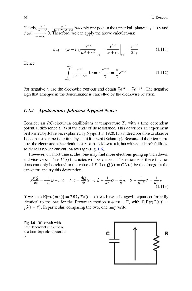
so there is no net current, on average (Fig. 1.6).
However, on short time scales, one may find more electrons going up than down,
and vice-versa. Thus U (t) fluctuates with zero mean. The variance of these fluctuations can only be related to the value of T . Let Q(t) = CU (t) be the charge in the
capacitor, and try this description:
R
dQ
dt
= −
1
C
Q + η(t); I (t) =
dQ
dt
(t) ⇒ ˙
Q +
1
RC
Q =
1
R
η; ˙
U +
1
RC 2 U =
1
RC
η
(1.113)
If we take E[η(t)η(t
)] = 2Rk B T δ(t − t
) we have a Langevin equation formally
identical to the one for the Brownian motion ˙
v + γv = , with E[(t))(t
)] =
qδ(t − t
). In particular, comparing the two, one may write:
Fig. 1.6 RC-circuit with
time dependent current due
to a time dependent potential
U
L. Rondoni
Clearly,
e
iωt
ω 2 +γ 2 =
e
iωt
(ω+iγ)(ω−iγ)
has only one pole in the upper half plane: w 0 = iγ and
f (ω) − −−− →
|ω|→∞
0. Therefore, we can apply the above calculations:
a −1 = (ω − iγ)
e
iωt
ω 2 + γ 2
iγ
=
e
iωt
ω + iγ
iγ
=
e
−γt
2iγ
(1.111)
Hence
+∞
−∞
e
iωt
ω 2 + γ 2 dω = π
e
−γt
γ
=
π
γ
e
−γt
(1.112)
For negative t, use the clockwise contour and obtain
π
γ
e
γt
=
π
γ
e
−γ|t| . The negative
sign that emerges in the denominator is cancelled by the clockwise rotation.
1.4.2 Application: Johnson-Nyquist Noise
Consider an RC-circuit in equilibrium at temperature T , with a time dependent
potential difference U (t) at the ends of its resistance. This describes an experiment
performed by Johnson, explained by Nyquist in 1928. It is indeed possible to observe
1 electron at a time is emitted by a hot filament (Schottky). Because of their temperature, the electrons in the cricuit move to up and down in it, but with equal probabilities,
so there is no net current, on average (Fig. 1.6).
However, on short time scales, one may find more electrons going up than down,
and vice-versa. Thus U (t) fluctuates with zero mean. The variance of these fluctuations can only be related to the value of T . Let Q(t) = CU (t) be the charge in the
capacitor, and try this description:
R
dQ
dt
= −
1
C
Q + η(t); I (t) =
dQ
dt
(t) ⇒ ˙
Q +
1
RC
Q =
1
R
η; ˙
U +
1
RC 2 U =
1
RC
η
(1.113)
If we take E[η(t)η(t
)] = 2Rk B T δ(t − t
) we have a Langevin equation formally
identical to the one for the Brownian motion ˙
v + γv = , with E[(t))(t
)] =
qδ(t − t
). In particular, comparing the two, one may write:
Fig. 1.6 RC-circuit with
time dependent current due
to a time dependent potential
U