

1 Introduction to Nonequilibrium Statistical Physics and Its Foundations
29
c
F(ω)
ω − ω 0
dω = 2πi F(ω 0 )
(1.103)
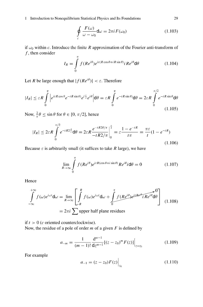
if ω 0 within c. Introduce the finite R approximation of the Fourier anti-transform of
f , then consider
I R =
π
0
f (Re
iθ
)e
it (R cos θ+i R sin θ) i Re
iθ dθ
(1.104)
Let R be large enough that | f (Re
iθ
)| < ε. Therefore
|I R | ≤ εR
π
0
e
it R cos θ e
−t R sin θ) e
i
π
2 e
iθ
dθ = εR
π
0
e
−t R sin θ) dθ = 2εR
π/2
0
e
−t R sin θ dθ
(1.105)
Now,
2
π
θ ≤ sin θ for θ ∈ [0, π/2], hence
|I R | ≤ 2εR
π/2
0
e
−t R2
θ
π dθ = 2εR
e
−t R2θ/π
−t R2/π
π
2
0
= ε
1 − e
−t R
tπ
=
πε
t
(1 − e
−t R
)
(1.106)
Because ε is arbitrarily small (it suffices to take R large), we have
lim
R→∞
π
0
f (Re
iθ
)e
it R(cos θ+i sin θ) Re
iθ idθ = 0
(1.107)
Hence
+∞
−∞
f (ω)e
iωt dω = lim
R→∞
⎡
⎣
R
−R
f (ω)e
iωt dω +
: 0
π
0
f (Re
iθ
)e
it Re
iθ i Re
iθ dθ
⎤
⎦
= 2πi
upper half plane residues
(1.108)
if t > 0 (c oriented counterclockwise).
Now, the residue of a pole of order m of a given F is defined by
a −m =
1
(m − 1)!
d
m−1
dz m−1 [(z − z 0 )
m F(z)]
z=z 0
(1.109)
For example
a −1 = (z − z 0 )F(z)
z 0
(1.110)
29
c
F(ω)
ω − ω 0
dω = 2πi F(ω 0 )
(1.103)
if ω 0 within c. Introduce the finite R approximation of the Fourier anti-transform of
f , then consider
I R =
π
0
f (Re
iθ
)e
it (R cos θ+i R sin θ) i Re
iθ dθ
(1.104)
Let R be large enough that | f (Re
iθ
)| < ε. Therefore
|I R | ≤ εR
π
0
e
it R cos θ e
−t R sin θ) e
i
π
2 e
iθ
dθ = εR
π
0
e
−t R sin θ) dθ = 2εR
π/2
0
e
−t R sin θ dθ
(1.105)
Now,
2
π
θ ≤ sin θ for θ ∈ [0, π/2], hence
|I R | ≤ 2εR
π/2
0
e
−t R2
θ
π dθ = 2εR
e
−t R2θ/π
−t R2/π
π
2
0
= ε
1 − e
−t R
tπ
=
πε
t
(1 − e
−t R
)
(1.106)
Because ε is arbitrarily small (it suffices to take R large), we have
lim
R→∞
π
0
f (Re
iθ
)e
it R(cos θ+i sin θ) Re
iθ idθ = 0
(1.107)
Hence
+∞
−∞
f (ω)e
iωt dω = lim
R→∞
⎡
⎣
R
−R
f (ω)e
iωt dω +
: 0
π
0
f (Re
iθ
)e
it Re
iθ i Re
iθ dθ
⎤
⎦
= 2πi
upper half plane residues
(1.108)
if t > 0 (c oriented counterclockwise).
Now, the residue of a pole of order m of a given F is defined by
a −m =
1
(m − 1)!
d
m−1
dz m−1 [(z − z 0 )
m F(z)]
z=z 0
(1.109)
For example
a −1 = (z − z 0 )F(z)
z 0
(1.110)