

28
L. Rondoni
If the Brownian particle has equilibrated with the fluid, equipartition of energy
applies, mE[v
2
] = k B T , hence
I =
γk B T
πm
(1.100)
in accord with Eq. (1.31).
Equation (1.100) states that the power of the random force is proprtional to the
friction coefficient and to the thermal energy. In turn, Einstein’s relation (1.37) represents an inverse proportionality between the diffusion coefficient and the friction
coefficient. Both results demonstrate that the dissipation of energy caused by friction
is intimately related to the equilibrium fluctuations, due to the incessant molecular
motions.
1.4.1 Exercise: Derivation of Eq. (1.98)
Consider the inverse F-transform of a given function f :
+∞
−∞
f (ω)e
iωt dω
(1.101)
where t ∈ R + and f is analytic in the upper half plane, except for a finite number of
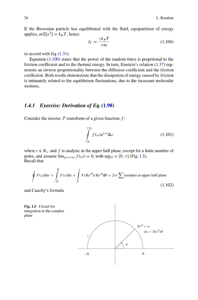
poles, and assume lim |ω|→∞ f (ω) = 0, with argω ∈ [0, π] (Fig. 1.5).
Recall that
c
F(ω)dw =
R
−R
F(x)dx +
π
0
F(Re
iθ )i Re
iθ dθ = 2πi
residues in upper half plane
(1.102)
and Cauchy’s formula
Fig. 1.5 Circuit for
integration in the complex
plane
L. Rondoni
If the Brownian particle has equilibrated with the fluid, equipartition of energy
applies, mE[v
2
] = k B T , hence
I =
γk B T
πm
(1.100)
in accord with Eq. (1.31).
Equation (1.100) states that the power of the random force is proprtional to the
friction coefficient and to the thermal energy. In turn, Einstein’s relation (1.37) represents an inverse proportionality between the diffusion coefficient and the friction
coefficient. Both results demonstrate that the dissipation of energy caused by friction
is intimately related to the equilibrium fluctuations, due to the incessant molecular
motions.
1.4.1 Exercise: Derivation of Eq. (1.98)
Consider the inverse F-transform of a given function f :
+∞
−∞
f (ω)e
iωt dω
(1.101)
where t ∈ R + and f is analytic in the upper half plane, except for a finite number of
poles, and assume lim |ω|→∞ f (ω) = 0, with argω ∈ [0, π] (Fig. 1.5).
Recall that
c
F(ω)dw =
R
−R
F(x)dx +
π
0
F(Re
iθ )i Re
iθ dθ = 2πi
residues in upper half plane
(1.102)
and Cauchy’s formula
Fig. 1.5 Circuit for
integration in the complex
plane