

5 Basics of Molecular Modeling and Molecular Simulation
235
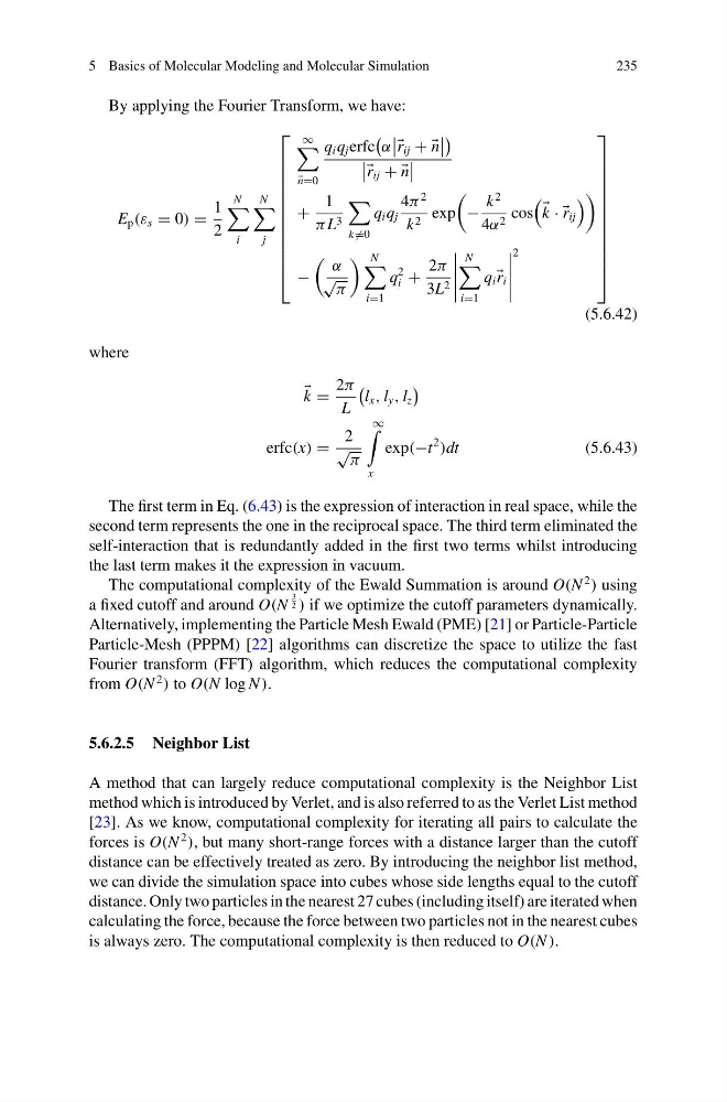
By applying the Fourier Transform, we have:
E p (ε s = 0) =
1
2
N
i
N
j
⎡
⎢
⎢
⎢
⎢
⎢
⎢
⎢
⎢
⎢
⎢
⎢
⎣
∞
n=0
q i q j erfc
α
r ij + +
n
r ij + +
n
+
1
π L 3
k =0
q i q j
4π
2
k 2 exp
−
k
2
4α 2 cos
k · · r ij
−
α
√
π
N
i=1
q
2
i +
2π
3L 2
N
i=1
q i r i
2
⎤
⎥
⎥
⎥
⎥
⎥
⎥
⎥
⎥
⎥
⎥
⎥
⎦
(5.6.42)
where
k =
2π
L
l x , l y , l z
erfc(x) =
2
√
π
∞
x
exp(−t
2
)dt
(5.6.43)
The first term in Eq. (6.43) is the expression of interaction in real space, while the
second term represents the one in the reciprocal space. The third term eliminated the
self-interaction that is redundantly added in the first two terms whilst introducing
the last term makes it the expression in vacuum.
The computational complexity of the Ewald Summation is around O(N
2
) using
a fixed cutoff and around O(N
3
2 ) if we optimize the cutoff parameters dynamically.
Alternatively, implementing the Particle Mesh Ewald (PME) [21] or Particle-Particle
Particle-Mesh (PPPM) [22] algorithms can discretize the space to utilize the fast
Fourier transform (FFT) algorithm, which reduces the computational complexity
from O(N
2
) to O(N log N ).
5.6.2.5 Neighbor List
A method that can largely reduce computational complexity is the Neighbor List
method which is introduced by Verlet, and is also referred to as the Verlet List method
[23]. As we know, computational complexity for iterating all pairs to calculate the
forces is O(N
2
), but many short-range forces with a distance larger than the cutoff
distance can be effectively treated as zero. By introducing the neighbor list method,
we can divide the simulation space into cubes whose side lengths equal to the cutoff
distance. Only two particles in the nearest 27 cubes (including itself) are iterated when
calculating the force, because the force between two particles not in the nearest cubes
is always zero. The computational complexity is then reduced to O(N ).
235
By applying the Fourier Transform, we have:
E p (ε s = 0) =
1
2
N
i
N
j
⎡
⎢
⎢
⎢
⎢
⎢
⎢
⎢
⎢
⎢
⎢
⎢
⎣
∞
n=0
q i q j erfc
α
r ij + +
n
r ij + +
n
+
1
π L 3
k =0
q i q j
4π
2
k 2 exp
−
k
2
4α 2 cos
k · · r ij
−
α
√
π
N
i=1
q
2
i +
2π
3L 2
N
i=1
q i r i
2
⎤
⎥
⎥
⎥
⎥
⎥
⎥
⎥
⎥
⎥
⎥
⎥
⎦
(5.6.42)
where
k =
2π
L
l x , l y , l z
erfc(x) =
2
√
π
∞
x
exp(−t
2
)dt
(5.6.43)
The first term in Eq. (6.43) is the expression of interaction in real space, while the
second term represents the one in the reciprocal space. The third term eliminated the
self-interaction that is redundantly added in the first two terms whilst introducing
the last term makes it the expression in vacuum.
The computational complexity of the Ewald Summation is around O(N
2
) using
a fixed cutoff and around O(N
3
2 ) if we optimize the cutoff parameters dynamically.
Alternatively, implementing the Particle Mesh Ewald (PME) [21] or Particle-Particle
Particle-Mesh (PPPM) [22] algorithms can discretize the space to utilize the fast
Fourier transform (FFT) algorithm, which reduces the computational complexity
from O(N
2
) to O(N log N ).
5.6.2.5 Neighbor List
A method that can largely reduce computational complexity is the Neighbor List
method which is introduced by Verlet, and is also referred to as the Verlet List method
[23]. As we know, computational complexity for iterating all pairs to calculate the
forces is O(N
2
), but many short-range forces with a distance larger than the cutoff
distance can be effectively treated as zero. By introducing the neighbor list method,
we can divide the simulation space into cubes whose side lengths equal to the cutoff
distance. Only two particles in the nearest 27 cubes (including itself) are iterated when
calculating the force, because the force between two particles not in the nearest cubes
is always zero. The computational complexity is then reduced to O(N ).