

234
C. Tang (唐晨宇) and Y. Wang (王延颋)
d r i
dt
=
p i
m i
1
s
ds
dt
= ζ
d
p i
dt
= −
∂E p ( r
N
)
∂ r i
− ς
p i
d
dt ζ =
i
p
2
i
m i
−
1
β
Q
H Nose =
N
i=1
p
2
i
2m i
+ E p ( r
N
) +
1
2
ς Q +
l
β
ln s, l = 3N
(5.6.39)
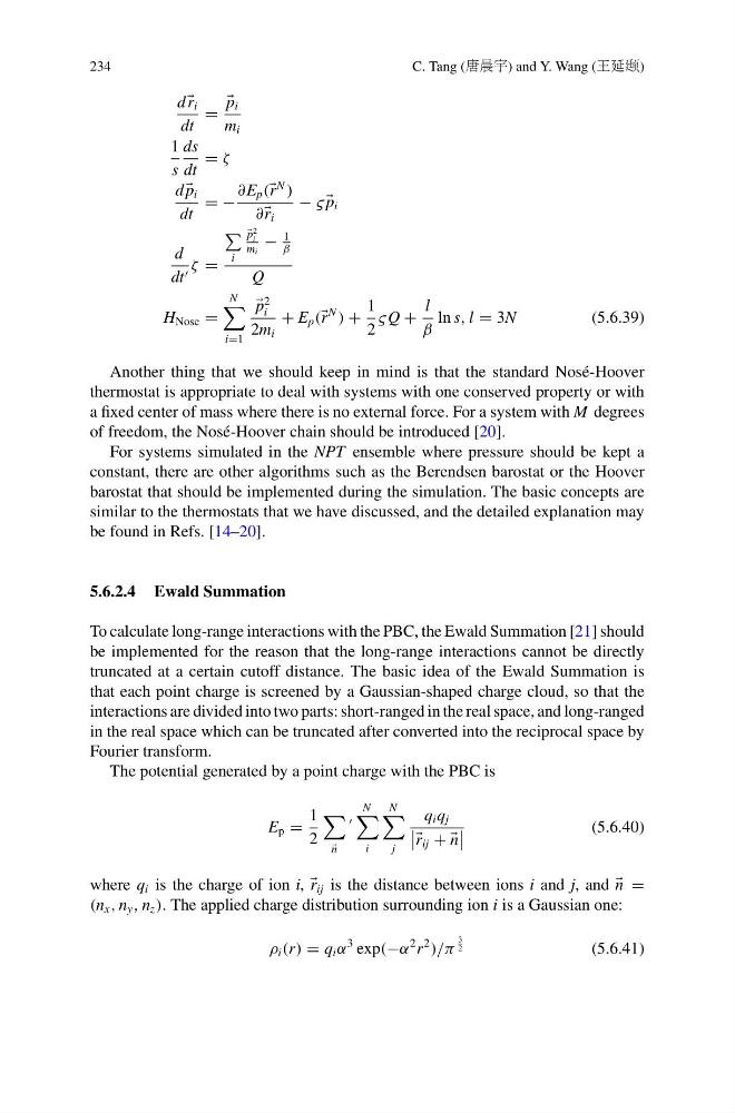
Another thing that we should keep in mind is that the standard Nosé-Hoover
thermostat is appropriate to deal with systems with one conserved property or with
a fixed center of mass where there is no external force. For a system with M degrees
of freedom, the Nosé-Hoover chain should be introduced [20].
For systems simulated in the NPT ensemble where pressure should be kept a
constant, there are other algorithms such as the Berendsen barostat or the Hoover
barostat that should be implemented during the simulation. The basic concepts are
similar to the thermostats that we have discussed, and the detailed explanation may
be found in Refs. [14–20].
5.6.2.4 Ewald Summation
To calculate long-range interactions with the PBC, the Ewald Summation [21] should
be implemented for the reason that the long-range interactions cannot be directly
truncated at a certain cutoff distance. The basic idea of the Ewald Summation is
that each point charge is screened by a Gaussian-shaped charge cloud, so that the
interactions are divided into two parts: short-ranged in the real space, and long-ranged
in the real space which can be truncated after converted into the reciprocal space by
Fourier transform.
The potential generated by a point charge with the PBC is
E p =
1
2
n
N
i
N
j
q i q j
r ij + +
n
(5.6.40)
where q i is the charge of ion i, r ij is the distance between ions i and j, and
n =
(n x , n y , n z ). The applied charge distribution surrounding ion i is a Gaussian one:
ρ i (r) = q i α
3 exp(−α
2 r
2
)/π
3
2
(5.6.41)
C. Tang (唐晨宇) and Y. Wang (王延颋)
d r i
dt
=
p i
m i
1
s
ds
dt
= ζ
d
p i
dt
= −
∂E p ( r
N
)
∂ r i
− ς
p i
d
dt ζ =
i
p
2
i
m i
−
1
β
Q
H Nose =
N
i=1
p
2
i
2m i
+ E p ( r
N
) +
1
2
ς Q +
l
β
ln s, l = 3N
(5.6.39)
Another thing that we should keep in mind is that the standard Nosé-Hoover
thermostat is appropriate to deal with systems with one conserved property or with
a fixed center of mass where there is no external force. For a system with M degrees
of freedom, the Nosé-Hoover chain should be introduced [20].
For systems simulated in the NPT ensemble where pressure should be kept a
constant, there are other algorithms such as the Berendsen barostat or the Hoover
barostat that should be implemented during the simulation. The basic concepts are
similar to the thermostats that we have discussed, and the detailed explanation may
be found in Refs. [14–20].
5.6.2.4 Ewald Summation
To calculate long-range interactions with the PBC, the Ewald Summation [21] should
be implemented for the reason that the long-range interactions cannot be directly
truncated at a certain cutoff distance. The basic idea of the Ewald Summation is
that each point charge is screened by a Gaussian-shaped charge cloud, so that the
interactions are divided into two parts: short-ranged in the real space, and long-ranged
in the real space which can be truncated after converted into the reciprocal space by
Fourier transform.
The potential generated by a point charge with the PBC is
E p =
1
2
n
N
i
N
j
q i q j
r ij + +
n
(5.6.40)
where q i is the charge of ion i, r ij is the distance between ions i and j, and
n =
(n x , n y , n z ). The applied charge distribution surrounding ion i is a Gaussian one:
ρ i (r) = q i α
3 exp(−α
2 r
2
)/π
3
2
(5.6.41)