

5 Basics of Molecular Modeling and Molecular Simulation
233
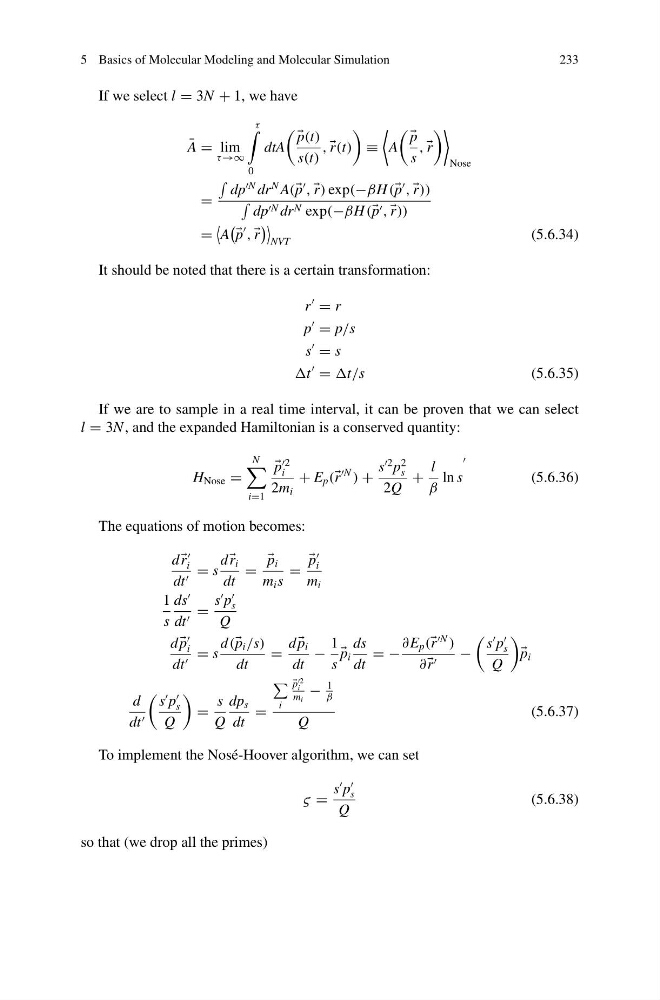
If we select l = 3N + 1, we have
¯
A = lim
τ →∞
τ
0
dtA
p(t)
s(t)
, r(t)
≡
A
p
s
, r
Nose
=
dp
N dr
N A( p
, r) exp(−βH ( p
, r))
dp N dr N exp(−βH ( p , r))
=
A
p
, r
NVT
(5.6.34)
It should be noted that there is a certain transformation:
r
= r
p
= p/s
s
= s
t
= t/s
(5.6.35)
If we are to sample in a real time interval, it can be proven that we can select
l = 3N , and the expanded Hamiltonian is a conserved quantity:
H Nose =
N
i=1
p
2
i
2m i
+ E p ( r
N
) +
s
2 p
2
s
2Q
+
l
β
ln s
(5.6.36)
The equations of motion becomes:
d r
i
dt = s
d r i
dt
=
p i
m i s
=
p
i
m i
1
s
ds
dt =
s
p
s
Q
d
p
i
dt = s
d ( p i /s)
dt
=
d
p i
dt
−
1
s
p i
ds
dt
= −
∂E p ( r
N
)
∂ r
−
s
p
s
Q
p i
d
dt
s
p
s
Q
=
s
Q
dp s
dt
=
i
p
2
i
m i
−
1
β
Q
(5.6.37)
To implement the Nosé-Hoover algorithm, we can set
ς =
s
p
s
Q
(5.6.38)
so that (we drop all the primes)
233
If we select l = 3N + 1, we have
¯
A = lim
τ →∞
τ
0
dtA
p(t)
s(t)
, r(t)
≡
A
p
s
, r
Nose
=
dp
N dr
N A( p
, r) exp(−βH ( p
, r))
dp N dr N exp(−βH ( p , r))
=
A
p
, r
NVT
(5.6.34)
It should be noted that there is a certain transformation:
r
= r
p
= p/s
s
= s
t
= t/s
(5.6.35)
If we are to sample in a real time interval, it can be proven that we can select
l = 3N , and the expanded Hamiltonian is a conserved quantity:
H Nose =
N
i=1
p
2
i
2m i
+ E p ( r
N
) +
s
2 p
2
s
2Q
+
l
β
ln s
(5.6.36)
The equations of motion becomes:
d r
i
dt = s
d r i
dt
=
p i
m i s
=
p
i
m i
1
s
ds
dt =
s
p
s
Q
d
p
i
dt = s
d ( p i /s)
dt
=
d
p i
dt
−
1
s
p i
ds
dt
= −
∂E p ( r
N
)
∂ r
−
s
p
s
Q
p i
d
dt
s
p
s
Q
=
s
Q
dp s
dt
=
i
p
2
i
m i
−
1
β
Q
(5.6.37)
To implement the Nosé-Hoover algorithm, we can set
ς =
s
p
s
Q
(5.6.38)
so that (we drop all the primes)