

5 Basics of Molecular Modeling and Molecular Simulation
225
5.6.2 MD Simulation and Sampling
As we have discussed earlier, the MD method simulates many-body systems through
solving many-body Newton’s Equations of Motion by calculating the resultant force
on each particle. The basic process of the MD simulation is illustrated in Fig. 5.3.
Some details of the simulation algorithms and related concepts will be illustrated in
the following parts.
5.6.2.1 Basic Concepts
Before digging into details of the simulation process, it is beneficial to clarify some
basic concepts that are normally introduced in MD simulations.
It is understandable that the simulation should be conducted in a limited space
within a limited time scale. Thus, the simulation space should be given first. The
continuity of simulation space can be either discrete, for instance, the space for the
Ising Model, or continuous. The Boundary Condition for the space can be either
free, rigid, or periodic. Among them, the most widely used and thus most important
boundary condition is the periodic boundary condition (PBC), under which particles
in the simulated box can interact with an infinite number of their images, allowing
us to study physical properties of macroscopic systems with ∼ 10
23 particles by
simulating only ∼ 10
3 to ∼ 10
6 particles. The total energy of a system simulated
with the PBC becomes:
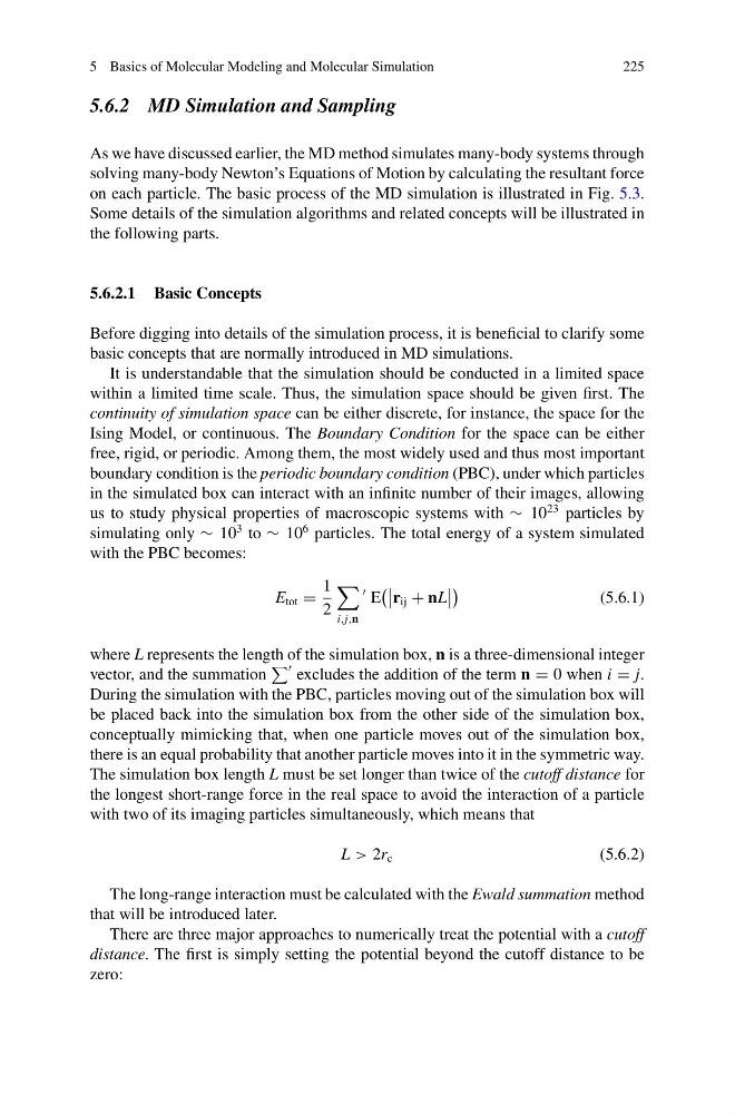
E tot =
1
2
i,j,n
E
r ij + nL
(5.6.1)
where L represents the length of the simulation box, n is a three-dimensional integer
vector, and the summation
excludes the addition of the term n = 0 when i = j.
During the simulation with the PBC, particles moving out of the simulation box will
be placed back into the simulation box from the other side of the simulation box,
conceptually mimicking that, when one particle moves out of the simulation box,
there is an equal probability that another particle moves into it in the symmetric way.
The simulation box length L must be set longer than twice of the cutoff distance for
the longest short-range force in the real space to avoid the interaction of a particle
with two of its imaging particles simultaneously, which means that
L > 2r c
(5.6.2)
The long-range interaction must be calculated with the Ewald summation method
that will be introduced later.
There are three major approaches to numerically treat the potential with a cutoff
distance. The first is simply setting the potential beyond the cutoff distance to be
zero:
225
5.6.2 MD Simulation and Sampling
As we have discussed earlier, the MD method simulates many-body systems through
solving many-body Newton’s Equations of Motion by calculating the resultant force
on each particle. The basic process of the MD simulation is illustrated in Fig. 5.3.
Some details of the simulation algorithms and related concepts will be illustrated in
the following parts.
5.6.2.1 Basic Concepts
Before digging into details of the simulation process, it is beneficial to clarify some
basic concepts that are normally introduced in MD simulations.
It is understandable that the simulation should be conducted in a limited space
within a limited time scale. Thus, the simulation space should be given first. The
continuity of simulation space can be either discrete, for instance, the space for the
Ising Model, or continuous. The Boundary Condition for the space can be either
free, rigid, or periodic. Among them, the most widely used and thus most important
boundary condition is the periodic boundary condition (PBC), under which particles
in the simulated box can interact with an infinite number of their images, allowing
us to study physical properties of macroscopic systems with ∼ 10
23 particles by
simulating only ∼ 10
3 to ∼ 10
6 particles. The total energy of a system simulated
with the PBC becomes:
E tot =
1
2
i,j,n
E
r ij + nL
(5.6.1)
where L represents the length of the simulation box, n is a three-dimensional integer
vector, and the summation
excludes the addition of the term n = 0 when i = j.
During the simulation with the PBC, particles moving out of the simulation box will
be placed back into the simulation box from the other side of the simulation box,
conceptually mimicking that, when one particle moves out of the simulation box,
there is an equal probability that another particle moves into it in the symmetric way.
The simulation box length L must be set longer than twice of the cutoff distance for
the longest short-range force in the real space to avoid the interaction of a particle
with two of its imaging particles simultaneously, which means that
L > 2r c
(5.6.2)
The long-range interaction must be calculated with the Ewald summation method
that will be introduced later.
There are three major approaches to numerically treat the potential with a cutoff
distance. The first is simply setting the potential beyond the cutoff distance to be
zero: