

5 Basics of Molecular Modeling and Molecular Simulation
219
come from the fact that, unlike reducing the degrees of freedom at the quantum level,
the adiabatic assumption usually does not work well at the atomistic level. Moreover, similar to atomistic force fields, different CG methods emphasize different
physical properties and loosen the accuracy for other properties. A CG method
normally requires either fitting from experimental and/or atomistic simulation data or
converting mathematically from the atomistic force field. Two typical CG methods
of the latter are the Multiscale Coarse-Graining (MS-CG) method and the Effective Force Coarse-Graining (EF-CG) method, both present researchers with tools
that reduce degrees of freedom and accelerate dynamics while containing necessary physical properties in chemical and biomolecular systems. The MARTINI CG
force field is a widely used general-purpose one developed for biomolecular systems.
Detailed explanations on their mechanism and applicability can be found in Refs.
[4–6].
5.5 Monte Carlo (MC) Simulation
5.5.1 Purpose
In the previous sections, we have brought forward some basic concepts of thermodynamics and classical statistical mechanics. To introduce the MC method, we can start
from the classical expression of the partition function Z, which has been introduced
in Sect. 3.2. For a system with N identical atoms in the canonical ensemble, the
partition function becomes:
Z =
1
h dN N !
d p
N d r
N exp
−βE(r 1 , r 2 , r 3 . . . r N , p 1 , p 2 , p 3 . . . p N )
(5.5.1)
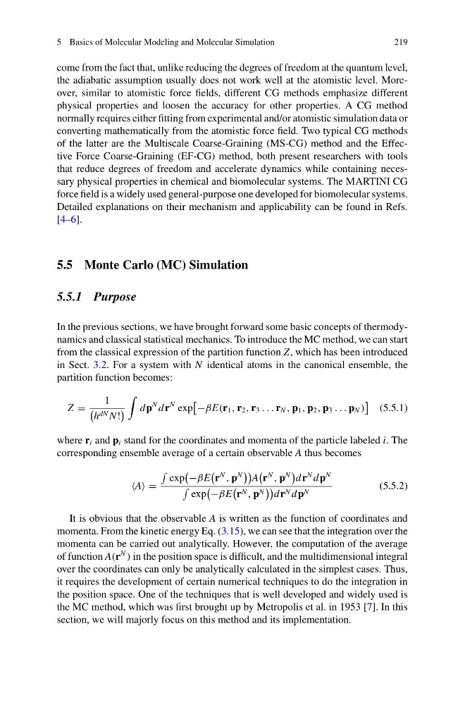
where r i and p i stand for the coordinates and momenta of the particle labeled i. The
corresponding ensemble average of a certain observable A thus becomes
A =
exp
−βE
r
N
, p
N
A
r
N
, p
N
d r
N d p
N
exp
−βE
r N , p N
d r N d p N
(5.5.2)
It is obvious that the observable A is written as the function of coordinates and
momenta. From the kinetic energy Eq. (3.15), we can see that the integration over the
momenta can be carried out analytically. However, the computation of the average
of function A(r
N
) in the position space is difficult, and the multidimensional integral
over the coordinates can only be analytically calculated in the simplest cases. Thus,
it requires the development of certain numerical techniques to do the integration in
the position space. One of the techniques that is well developed and widely used is
the MC method, which was first brought up by Metropolis et al. in 1953 [7]. In this
section, we will majorly focus on this method and its implementation.
219
come from the fact that, unlike reducing the degrees of freedom at the quantum level,
the adiabatic assumption usually does not work well at the atomistic level. Moreover, similar to atomistic force fields, different CG methods emphasize different
physical properties and loosen the accuracy for other properties. A CG method
normally requires either fitting from experimental and/or atomistic simulation data or
converting mathematically from the atomistic force field. Two typical CG methods
of the latter are the Multiscale Coarse-Graining (MS-CG) method and the Effective Force Coarse-Graining (EF-CG) method, both present researchers with tools
that reduce degrees of freedom and accelerate dynamics while containing necessary physical properties in chemical and biomolecular systems. The MARTINI CG
force field is a widely used general-purpose one developed for biomolecular systems.
Detailed explanations on their mechanism and applicability can be found in Refs.
[4–6].
5.5 Monte Carlo (MC) Simulation
5.5.1 Purpose
In the previous sections, we have brought forward some basic concepts of thermodynamics and classical statistical mechanics. To introduce the MC method, we can start
from the classical expression of the partition function Z, which has been introduced
in Sect. 3.2. For a system with N identical atoms in the canonical ensemble, the
partition function becomes:
Z =
1
h dN N !
d p
N d r
N exp
−βE(r 1 , r 2 , r 3 . . . r N , p 1 , p 2 , p 3 . . . p N )
(5.5.1)
where r i and p i stand for the coordinates and momenta of the particle labeled i. The
corresponding ensemble average of a certain observable A thus becomes
A =
exp
−βE
r
N
, p
N
A
r
N
, p
N
d r
N d p
N
exp
−βE
r N , p N
d r N d p N
(5.5.2)
It is obvious that the observable A is written as the function of coordinates and
momenta. From the kinetic energy Eq. (3.15), we can see that the integration over the
momenta can be carried out analytically. However, the computation of the average
of function A(r
N
) in the position space is difficult, and the multidimensional integral
over the coordinates can only be analytically calculated in the simplest cases. Thus,
it requires the development of certain numerical techniques to do the integration in
the position space. One of the techniques that is well developed and widely used is
the MC method, which was first brought up by Metropolis et al. in 1953 [7]. In this
section, we will majorly focus on this method and its implementation.