

220
C. Tang (唐晨宇) and Y. Wang (王延颋)
5.5.2 Importance Sampling
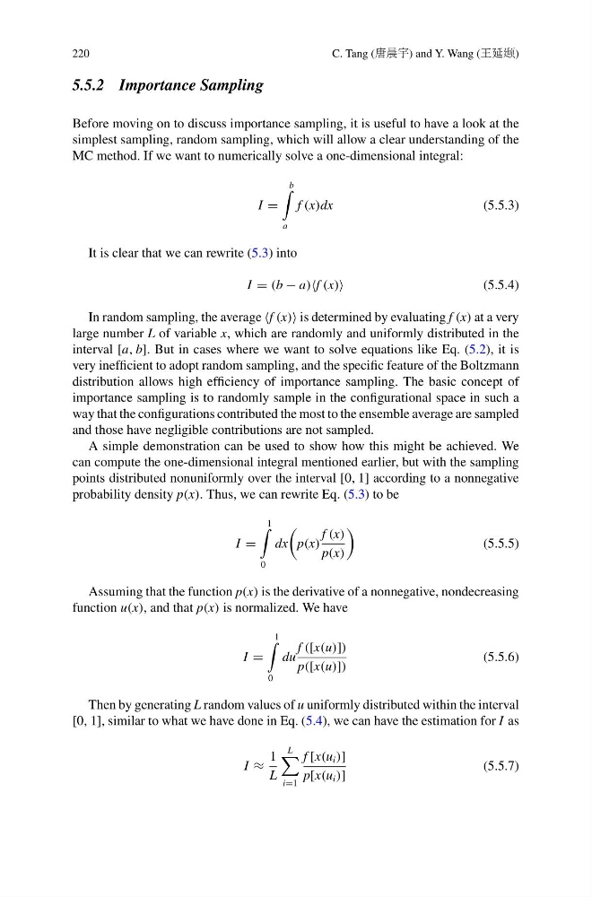
Before moving on to discuss importance sampling, it is useful to have a look at the
simplest sampling, random sampling, which will allow a clear understanding of the
MC method. If we want to numerically solve a one-dimensional integral:
I =
b
a
f (x)dx
(5.5.3)
It is clear that we can rewrite (5.3) into
I = (b − a)f (x)
(5.5.4)
In random sampling, the average f (x) is determined by evaluating f (x) at a very
large number L of variable x, which are randomly and uniformly distributed in the
interval [a, b]. But in cases where we want to solve equations like Eq. (5.2), it is
very inefficient to adopt random sampling, and the specific feature of the Boltzmann
distribution allows high efficiency of importance sampling. The basic concept of
importance sampling is to randomly sample in the configurational space in such a
way that the configurations contributed the most to the ensemble average are sampled
and those have negligible contributions are not sampled.
A simple demonstration can be used to show how this might be achieved. We
can compute the one-dimensional integral mentioned earlier, but with the sampling
points distributed nonuniformly over the interval [0, 1] according to a nonnegative
probability density p(x). Thus, we can rewrite Eq. (5.3) to be
I =
1
0
dx
p(x)
f (x)
p(x)
(5.5.5)
Assuming that the function p(x) is the derivative of a nonnegative, nondecreasing
function u(x), and that p(x) is normalized. We have
I =
1
0
du
f ([x(u)])
p([x(u)])
(5.5.6)
Then by generating L random values of u uniformly distributed within the interval
[0, 1], similar to what we have done in Eq. (5.4), we can have the estimation for I as
I ≈
1
L
L
i=1
f [x(u i )]
p[x(u i )]
(5.5.7)
C. Tang (唐晨宇) and Y. Wang (王延颋)
5.5.2 Importance Sampling
Before moving on to discuss importance sampling, it is useful to have a look at the
simplest sampling, random sampling, which will allow a clear understanding of the
MC method. If we want to numerically solve a one-dimensional integral:
I =
b
a
f (x)dx
(5.5.3)
It is clear that we can rewrite (5.3) into
I = (b − a)f (x)
(5.5.4)
In random sampling, the average f (x) is determined by evaluating f (x) at a very
large number L of variable x, which are randomly and uniformly distributed in the
interval [a, b]. But in cases where we want to solve equations like Eq. (5.2), it is
very inefficient to adopt random sampling, and the specific feature of the Boltzmann
distribution allows high efficiency of importance sampling. The basic concept of
importance sampling is to randomly sample in the configurational space in such a
way that the configurations contributed the most to the ensemble average are sampled
and those have negligible contributions are not sampled.
A simple demonstration can be used to show how this might be achieved. We
can compute the one-dimensional integral mentioned earlier, but with the sampling
points distributed nonuniformly over the interval [0, 1] according to a nonnegative
probability density p(x). Thus, we can rewrite Eq. (5.3) to be
I =
1
0
dx
p(x)
f (x)
p(x)
(5.5.5)
Assuming that the function p(x) is the derivative of a nonnegative, nondecreasing
function u(x), and that p(x) is normalized. We have
I =
1
0
du
f ([x(u)])
p([x(u)])
(5.5.6)
Then by generating L random values of u uniformly distributed within the interval
[0, 1], similar to what we have done in Eq. (5.4), we can have the estimation for I as
I ≈
1
L
L
i=1
f [x(u i )]
p[x(u i )]
(5.5.7)