

4 An Introduction to Emergence Dynamics in Complex Systems
175
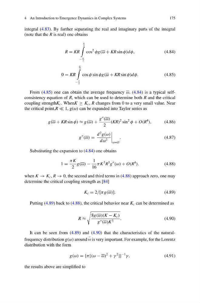
integral (4.83). By further separating the real and imaginary parts of the integral
(note that the R is real) one obtains
R = KR
π
2
−
π
2
cos
2
φg(ω + KR sin φ)d φ,
(4.84)
0 = KR
π
2
−
π
2
cos φ sin φg(ω + KR sin φ)d φ.
(4.85)
From (4.85) one can obtain the average frequency ω. (4.84) is a typical selfconsistency equation of R, which can be used to determine both R and the critical
coupling strengthK c . WhenK ≥ K c , R changes from 0 to a very small value. Near
the critical point,R 1, g(ω) can be expanded into Taylor series as
g(ω + KR sin φ) ≈ g(ω) +
g
(ω)
2
(KR)
2 sin
2
φ + O(R
4
),
(4.86)
g
(ω) =
d
2 g(ω)
d ω 2
ω=ω
.
(4.87)
Substituting the expansion to (4.84) one obtains
1 =
π K
2
g(ω) −
1
16
π K
3 R
3 g
(ω) + O(R
4
).
(4.88)
when K → K c , R → 0, the second and third terms in (4.88) approach zero, one may
determine the critical coupling strength as [84]
K c = 2/[π g(ω)].
(4.89)
Putting (4.89) back to (4.88), the critical behavior near K c can be determined as
R ≈
8g(ω)(K − K c )
g (ω)K 3
.
(4.90)
It can be seen from (4.89) and (4.90) that the characteristics of the naturalfrequency distribution g(ω) around
−
ω is very important. For example, for the Lorentz
distribution with the form
g(ω) = {π [(ω − ω)
2
+ γ
2
]}
−1
γ,
(4.91)
the results above are simplified to
175
integral (4.83). By further separating the real and imaginary parts of the integral
(note that the R is real) one obtains
R = KR
π
2
−
π
2
cos
2
φg(ω + KR sin φ)d φ,
(4.84)
0 = KR
π
2
−
π
2
cos φ sin φg(ω + KR sin φ)d φ.
(4.85)
From (4.85) one can obtain the average frequency ω. (4.84) is a typical selfconsistency equation of R, which can be used to determine both R and the critical
coupling strengthK c . WhenK ≥ K c , R changes from 0 to a very small value. Near
the critical point,R 1, g(ω) can be expanded into Taylor series as
g(ω + KR sin φ) ≈ g(ω) +
g
(ω)
2
(KR)
2 sin
2
φ + O(R
4
),
(4.86)
g
(ω) =
d
2 g(ω)
d ω 2
ω=ω
.
(4.87)
Substituting the expansion to (4.84) one obtains
1 =
π K
2
g(ω) −
1
16
π K
3 R
3 g
(ω) + O(R
4
).
(4.88)
when K → K c , R → 0, the second and third terms in (4.88) approach zero, one may
determine the critical coupling strength as [84]
K c = 2/[π g(ω)].
(4.89)
Putting (4.89) back to (4.88), the critical behavior near K c can be determined as
R ≈
8g(ω)(K − K c )
g (ω)K 3
.
(4.90)
It can be seen from (4.89) and (4.90) that the characteristics of the naturalfrequency distribution g(ω) around
−
ω is very important. For example, for the Lorentz
distribution with the form
g(ω) = {π [(ω − ω)
2
+ γ
2
]}
−1
γ,
(4.91)
the results above are simplified to