

176
Z. Zheng
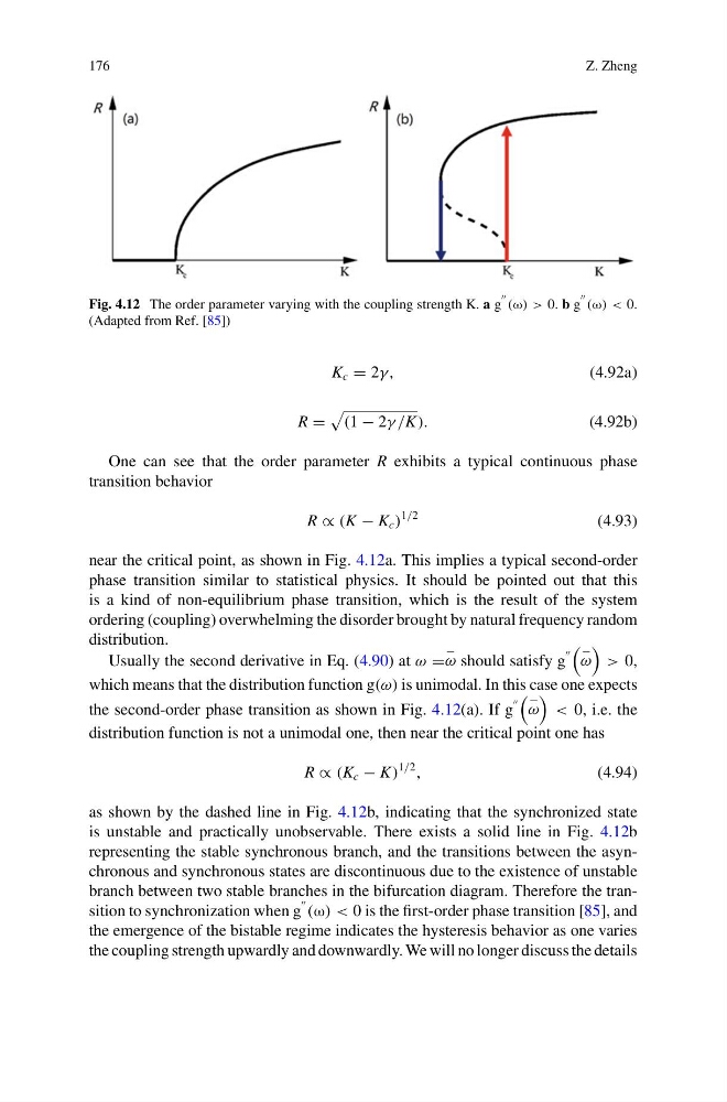
Fig. 4.12 The order parameter varying with the coupling strength K. a g
(ω) > 0. b g
(ω) < 0.
(Adapted from Ref. [85])
K c = 2γ,
(4.92a)
R =
(1 − 2γ /K).
(4.92b)
One can see that the order parameter R exhibits a typical continuous phase
transition behavior
R ∝ (K − K c )
1/2
(4.93)
near the critical point, as shown in Fig. 4.12a. This implies a typical second-order
phase transition similar to statistical physics. It should be pointed out that this
is a kind of non-equilibrium phase transition, which is the result of the system
ordering (coupling) overwhelming the disorder brought by natural frequency random
distribution.
Usually the second derivative in Eq. (4.90) at ω =
−
ω should satisfy g
−
ω
> 0,
which means that the distribution function g(ω) is unimodal. In this case one expects
the second-order phase transition as shown in Fig. 4.12(a). If g
−
ω
< 0, i.e. the
distribution function is not a unimodal one, then near the critical point one has
R ∝ (K c − K)
1/2
,
(4.94)
as shown by the dashed line in Fig. 4.12b, indicating that the synchronized state
is unstable and practically unobservable. There exists a solid line in Fig. 4.12b
representing the stable synchronous branch, and the transitions between the asynchronous and synchronous states are discontinuous due to the existence of unstable
branch between two stable branches in the bifurcation diagram. Therefore the transition to synchronization when g
(ω) < 0 is the first-order phase transition [85], and
the emergence of the bistable regime indicates the hysteresis behavior as one varies
the coupling strength upwardly and downwardly. We will no longer discuss the details
Z. Zheng
Fig. 4.12 The order parameter varying with the coupling strength K. a g
(ω) > 0. b g
(ω) < 0.
(Adapted from Ref. [85])
K c = 2γ,
(4.92a)
R =
(1 − 2γ /K).
(4.92b)
One can see that the order parameter R exhibits a typical continuous phase
transition behavior
R ∝ (K − K c )
1/2
(4.93)
near the critical point, as shown in Fig. 4.12a. This implies a typical second-order
phase transition similar to statistical physics. It should be pointed out that this
is a kind of non-equilibrium phase transition, which is the result of the system
ordering (coupling) overwhelming the disorder brought by natural frequency random
distribution.
Usually the second derivative in Eq. (4.90) at ω =
−
ω should satisfy g
−
ω
> 0,
which means that the distribution function g(ω) is unimodal. In this case one expects
the second-order phase transition as shown in Fig. 4.12(a). If g
−
ω
< 0, i.e. the
distribution function is not a unimodal one, then near the critical point one has
R ∝ (K c − K)
1/2
,
(4.94)
as shown by the dashed line in Fig. 4.12b, indicating that the synchronized state
is unstable and practically unobservable. There exists a solid line in Fig. 4.12b
representing the stable synchronous branch, and the transitions between the asynchronous and synchronous states are discontinuous due to the existence of unstable
branch between two stable branches in the bifurcation diagram. Therefore the transition to synchronization when g
(ω) < 0 is the first-order phase transition [85], and
the emergence of the bistable regime indicates the hysteresis behavior as one varies
the coupling strength upwardly and downwardly. We will no longer discuss the details