

4 An Introduction to Emergence Dynamics in Complex Systems
173
ξ i (t) = 0,
ξ i (t)ξ j (t
)
= Dδ ij δ(t − t
),
(4.70)
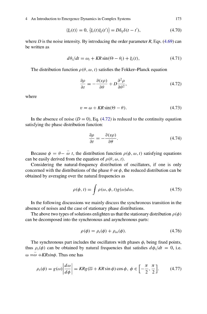
where D is the noise intensity. By introducing the order parameter R, Eqs. (4.69) can
be written as
d θ i /dt = ω i + KR sin(( − θ i ) + ξ i (t),
(4.71)
The distribution function ρ(θ, ω, t) satisfies the Fokker–Planck equation
∂ρ
∂t
= −
∂(vρ)
∂θ
+ D
∂
2
ρ
∂θ 2 ,
(4.72)
where
v = ω + KR sin(( − θ).
(4.73)
In the absence of noise (D = 0), Eq. (4.72) is reduced to the continuity equation
satisfying the phase distribution function:
∂ρ
∂t
= −
∂(vρ)
∂θ
.
(4.74)
Because φ = θ −
−
ω t, the distribution function ρ(φ, ω, t) satisfying equations
can be easily derived from the equation of ρ(θ, ω, t).
Considering the natural-frequency distribution of oscillators, if one is only
concerned with the distributions of the phase θ or φ, the reduced distribution can be
obtained by averaging over the natural frequencies as
ρ(φ, t) =
ρ(ω, φ, t)g(ω)d ω,
(4.75)
In the following discussions we mainly discuss the synchronous transition in the
absence of noises and the case of stationary phase distributions.
The above two types of solutions enlighten us that the stationary distribution ρ(φ)
can be decomposed into the synchronous and asynchronous parts:
ρ(φ) = ρ s (φ) + ρ as (φ).
(4.76)
The synchronous part includes the oscillators with phases φ i being fixed points,
thus ρ s (φ) can be obtained by natural frequencies that satisfies d φ i /dt = 0, i.e.
ω =
−
ω +KRsinφ. Thus one has
ρ s (φ) = g(ω)
d ω
d φ
= KRg(ω + KR sin φ) cos φ, φ ∈
−
π
2
,
π
2
.
(4.77)
173
ξ i (t) = 0,
ξ i (t)ξ j (t
)
= Dδ ij δ(t − t
),
(4.70)
where D is the noise intensity. By introducing the order parameter R, Eqs. (4.69) can
be written as
d θ i /dt = ω i + KR sin(( − θ i ) + ξ i (t),
(4.71)
The distribution function ρ(θ, ω, t) satisfies the Fokker–Planck equation
∂ρ
∂t
= −
∂(vρ)
∂θ
+ D
∂
2
ρ
∂θ 2 ,
(4.72)
where
v = ω + KR sin(( − θ).
(4.73)
In the absence of noise (D = 0), Eq. (4.72) is reduced to the continuity equation
satisfying the phase distribution function:
∂ρ
∂t
= −
∂(vρ)
∂θ
.
(4.74)
Because φ = θ −
−
ω t, the distribution function ρ(φ, ω, t) satisfying equations
can be easily derived from the equation of ρ(θ, ω, t).
Considering the natural-frequency distribution of oscillators, if one is only
concerned with the distributions of the phase θ or φ, the reduced distribution can be
obtained by averaging over the natural frequencies as
ρ(φ, t) =
ρ(ω, φ, t)g(ω)d ω,
(4.75)
In the following discussions we mainly discuss the synchronous transition in the
absence of noises and the case of stationary phase distributions.
The above two types of solutions enlighten us that the stationary distribution ρ(φ)
can be decomposed into the synchronous and asynchronous parts:
ρ(φ) = ρ s (φ) + ρ as (φ).
(4.76)
The synchronous part includes the oscillators with phases φ i being fixed points,
thus ρ s (φ) can be obtained by natural frequencies that satisfies d φ i /dt = 0, i.e.
ω =
−
ω +KRsinφ. Thus one has
ρ s (φ) = g(ω)
d ω
d φ
= KRg(ω + KR sin φ) cos φ, φ ∈
−
π
2
,
π
2
.
(4.77)