

4 An Introduction to Emergence Dynamics in Complex Systems
169
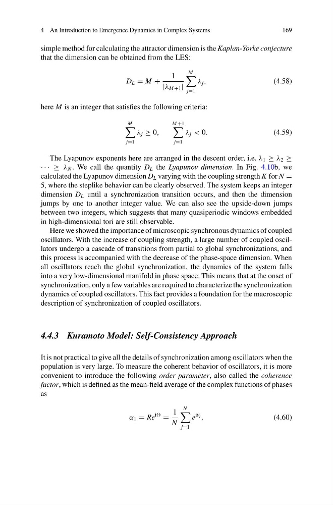
simple method for calculating the attractor dimension is the Kaplan-Yorke conjecture
that the dimension can be obtained from the LES:
D L = M +
1
|λ M +1 |
M
j=1
λ j ,
(4.58)
here M is an integer that satisfies the following criteria:
M
j=1
λ j ≥ 0,
M +1
j=1
λ j < 0.
(4.59)
The Lyapunov exponents here are arranged in the descent order, i.e. λ 1 ≥ λ 2 ≥
· · · ≥ λ N . We call the quantity D L the Lyapunov dimension. In Fig. 4.10b, we
calculated the Lyapunov dimension D L varying with the coupling strength K for N =
5, where the steplike behavior can be clearly observed. The system keeps an integer
dimension D L until a synchronization transition occurs, and then the dimension
jumps by one to another integer value. We can also see the upside-down jumps
between two integers, which suggests that many quasiperiodic windows embedded
in high-dimensional tori are still observable.
Here we showed the importance of microscopic synchronous dynamics of coupled
oscillators. With the increase of coupling strength, a large number of coupled oscillators undergo a cascade of transitions from partial to global synchronizations, and
this process is accompanied with the decrease of the phase-space dimension. When
all oscillators reach the global synchronization, the dynamics of the system falls
into a very low-dimensional manifold in phase space. This means that at the onset of
synchronization, only a few variables are required to characterize the synchronization
dynamics of coupled oscillators. This fact provides a foundation for the macroscopic
description of synchronization of coupled oscillators.
4.4.3 Kuramoto Model: Self-Consistency Approach
It is not practical to give all the details of synchronization among oscillators when the
population is very large. To measure the coherent behavior of oscillators, it is more
convenient to introduce the following order parameter, also called the coherence
factor, which is defined as the mean-field average of the complex functions of phases
as
α 1 = Re
i
=
1
N
N
j=1
e
iθ j .
(4.60)
169
simple method for calculating the attractor dimension is the Kaplan-Yorke conjecture
that the dimension can be obtained from the LES:
D L = M +
1
|λ M +1 |
M
j=1
λ j ,
(4.58)
here M is an integer that satisfies the following criteria:
M
j=1
λ j ≥ 0,
M +1
j=1
λ j < 0.
(4.59)
The Lyapunov exponents here are arranged in the descent order, i.e. λ 1 ≥ λ 2 ≥
· · · ≥ λ N . We call the quantity D L the Lyapunov dimension. In Fig. 4.10b, we
calculated the Lyapunov dimension D L varying with the coupling strength K for N =
5, where the steplike behavior can be clearly observed. The system keeps an integer
dimension D L until a synchronization transition occurs, and then the dimension
jumps by one to another integer value. We can also see the upside-down jumps
between two integers, which suggests that many quasiperiodic windows embedded
in high-dimensional tori are still observable.
Here we showed the importance of microscopic synchronous dynamics of coupled
oscillators. With the increase of coupling strength, a large number of coupled oscillators undergo a cascade of transitions from partial to global synchronizations, and
this process is accompanied with the decrease of the phase-space dimension. When
all oscillators reach the global synchronization, the dynamics of the system falls
into a very low-dimensional manifold in phase space. This means that at the onset of
synchronization, only a few variables are required to characterize the synchronization
dynamics of coupled oscillators. This fact provides a foundation for the macroscopic
description of synchronization of coupled oscillators.
4.4.3 Kuramoto Model: Self-Consistency Approach
It is not practical to give all the details of synchronization among oscillators when the
population is very large. To measure the coherent behavior of oscillators, it is more
convenient to introduce the following order parameter, also called the coherence
factor, which is defined as the mean-field average of the complex functions of phases
as
α 1 = Re
i
=
1
N
N
j=1
e
iθ j .
(4.60)