

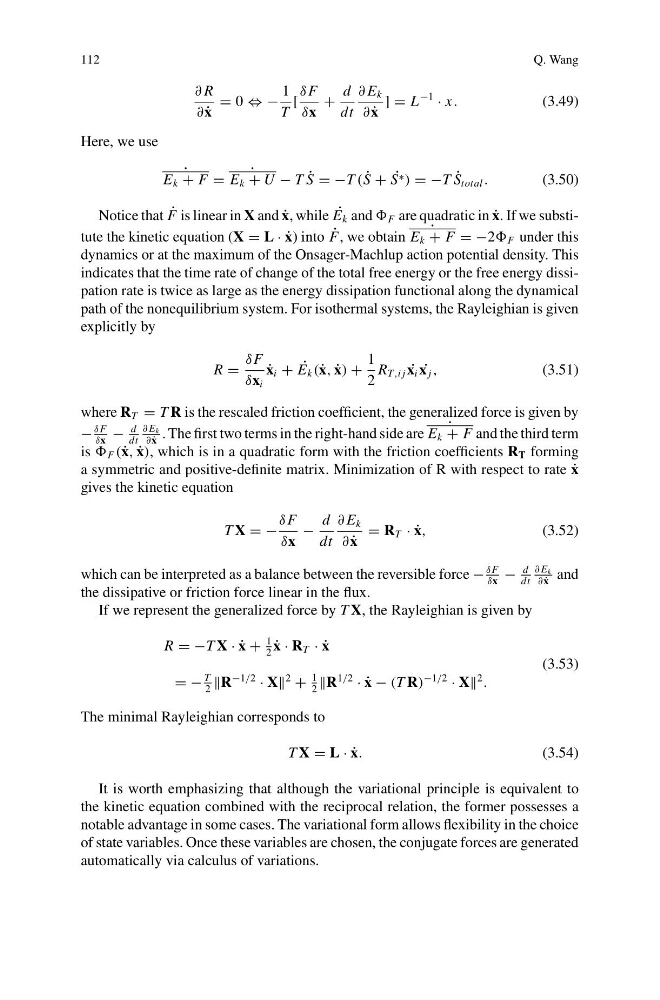
112
Q. Wang
∂ R
∂ ˙
x
= 0 ⇔ −
1
T
[
δ F
δx
+
d
dt
∂ E k
∂ ˙
x
] = L
−1
· x.
(3.49)
Here, we use
˙
E k + F =
˙
E k + U − T ˙
S = −T ( ˙
S + ˙
S ∗ ) = −T ˙
S total .
(3.50)
Notice that ˙
F is linear in X and ˙
x, while ˙
E k and F are quadratic in ˙
x. If we substitute the kinetic equation (X = L · ˙
x) into ˙
F, we obtain
˙
E k + F = −2 F under this
dynamics or at the maximum of the Onsager-Machlup action potential density. This
indicates that the time rate of change of the total free energy or the free energy dissipation rate is twice as large as the energy dissipation functional along the dynamical
path of the nonequilibrium system. For isothermal systems, the Rayleighian is given
explicitly by
R =
δ F
δx i
˙
x i + ˙
E k (˙ x, ˙
x) +
1
2
R T,i j ˙
x i ˙
x j ,
(3.51)
where R T = T R is the rescaled friction coefficient, the generalized force is given by
−
δ F
δx
−
d
dt
∂ E k
∂ ˙
x
. The first two terms in the right-hand side are
˙
E k + F and the third term
is F (˙ x, ˙
x), which is in a quadratic form with the friction coefficients R T forming
a symmetric and positive-definite matrix. Minimization of R with respect to rate ˙
x
gives the kinetic equation
T X = −
δ F
δx
−
d
dt
∂ E k
∂ ˙
x
= R T · ˙
x,
(3.52)
which can be interpreted as a balance between the reversible force −
δ F
δx
−
d
dt
∂ E k
∂ ˙
x
and
the dissipative or friction force linear in the flux.
If we represent the generalized force by T X, the Rayleighian is given by
R = −T X · ˙
x +
1
2
˙
x · R T · ˙
x
= −
T
2
R
−1/2
· X
2
+
1
2
R
1/2
· ˙
x − (T R)
−1/2
· X
2
.
(3.53)
The minimal Rayleighian corresponds to
T X = L · ˙
x.
(3.54)
It is worth emphasizing that although the variational principle is equivalent to
the kinetic equation combined with the reciprocal relation, the former possesses a
notable advantage in some cases. The variational form allows flexibility in the choice
of state variables. Once these variables are chosen, the conjugate forces are generated
automatically via calculus of variations.
Q. Wang
∂ R
∂ ˙
x
= 0 ⇔ −
1
T
[
δ F
δx
+
d
dt
∂ E k
∂ ˙
x
] = L
−1
· x.
(3.49)
Here, we use
˙
E k + F =
˙
E k + U − T ˙
S = −T ( ˙
S + ˙
S ∗ ) = −T ˙
S total .
(3.50)
Notice that ˙
F is linear in X and ˙
x, while ˙
E k and F are quadratic in ˙
x. If we substitute the kinetic equation (X = L · ˙
x) into ˙
F, we obtain
˙
E k + F = −2 F under this
dynamics or at the maximum of the Onsager-Machlup action potential density. This
indicates that the time rate of change of the total free energy or the free energy dissipation rate is twice as large as the energy dissipation functional along the dynamical
path of the nonequilibrium system. For isothermal systems, the Rayleighian is given
explicitly by
R =
δ F
δx i
˙
x i + ˙
E k (˙ x, ˙
x) +
1
2
R T,i j ˙
x i ˙
x j ,
(3.51)
where R T = T R is the rescaled friction coefficient, the generalized force is given by
−
δ F
δx
−
d
dt
∂ E k
∂ ˙
x
. The first two terms in the right-hand side are
˙
E k + F and the third term
is F (˙ x, ˙
x), which is in a quadratic form with the friction coefficients R T forming
a symmetric and positive-definite matrix. Minimization of R with respect to rate ˙
x
gives the kinetic equation
T X = −
δ F
δx
−
d
dt
∂ E k
∂ ˙
x
= R T · ˙
x,
(3.52)
which can be interpreted as a balance between the reversible force −
δ F
δx
−
d
dt
∂ E k
∂ ˙
x
and
the dissipative or friction force linear in the flux.
If we represent the generalized force by T X, the Rayleighian is given by
R = −T X · ˙
x +
1
2
˙
x · R T · ˙
x
= −
T
2
R
−1/2
· X
2
+
1
2
R
1/2
· ˙
x − (T R)
−1/2
· X
2
.
(3.53)
The minimal Rayleighian corresponds to
T X = L · ˙
x.
(3.54)
It is worth emphasizing that although the variational principle is equivalent to
the kinetic equation combined with the reciprocal relation, the former possesses a
notable advantage in some cases. The variational form allows flexibility in the choice
of state variables. Once these variables are chosen, the conjugate forces are generated
automatically via calculus of variations.