

3 Generalized Onsager Principle and It Applications
111
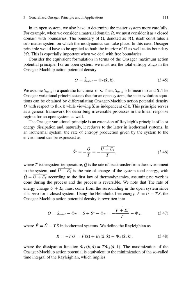
In an open system, we also have to determine the matter system more carefully.
For example, when we consider a material domain , we must consider it as a closed
domain with boundaries. The boundary of , denoted as ∂∂, itself constitutes a
sub-matter system on which thermodynamics can take place. In this case, Onsager
principle would have to be applied to both the interior of as well as its boundary
∂∂, This is especially important when we deal with free boundaries.
Consider the equivalent formulation in terms of the Onsager maximum action
potential principle. For an open system, we must use the total entropy S total in the
Onsager-Machlup action potential density
O = ˙
S total − S (˙ x, ˙
x).
(3.45)
We assume S total is a quadratic functional of x. Then, ˙
S total is bilinear in ˙
x and X. The
Onsager variational principle states that for an open system, the state evolution equations can be obtained by differentiating Onsager-Machlup action potential density
O with respect to flux ˙
x while viewing X as independent of ˙
x. This principle serves
as a general framework for describing irreversible processes in the linear response
regime for an open system as well.
The Onsager variational principle is an extension of Rayleigh’s principle of least
energy dissipation and, naturally, it reduces to the latter in isothermal systems. In
an isothermal system, the rate of entropy production given by the system to the
environment can be expressed as
˙
S ∗ = −
˙
Q
T
= −
˙
U + E k
T
,
(3.46)
where T is the system temperature, ˙
Q is the rate of heat transfer from the environment
to the system, and
˙
U + E k is the rate of change of the system total energy, with
˙
Q =
˙
U + E k according to the first law of thermodynamics, assuming no work is
done during the process and the process is reversible. We note that The rate of
energy change
˙
U + E k must come from the surrounding in the open system since
it is zero for a closed system. Using the Helmholtz free energy, F = U − T S, the
Onsager-Machlup action potential density is rewritten into
O = ˙
S total − S = ˙
S + ˙
S ∗ − S = −
˙
F + E k
T
− S ,
(3.47)
where ˙
F = ˙
U − T ˙
S in isothermal systems. We define the Rayleighian as
R = −T O = ˙
F(x) + ˙
E k (˙ x, ˙
x) + F (˙ x, ˙
x),
(3.48)
where the dissipation function F (˙ x, ˙
x) = T S (˙ x, ˙
x). The maximization of the
Onsager-Machlup action potential is equivalent to the minimization of the so-called
time integral of the Rayleighian, which implies
111
In an open system, we also have to determine the matter system more carefully.
For example, when we consider a material domain , we must consider it as a closed
domain with boundaries. The boundary of , denoted as ∂∂, itself constitutes a
sub-matter system on which thermodynamics can take place. In this case, Onsager
principle would have to be applied to both the interior of as well as its boundary
∂∂, This is especially important when we deal with free boundaries.
Consider the equivalent formulation in terms of the Onsager maximum action
potential principle. For an open system, we must use the total entropy S total in the
Onsager-Machlup action potential density
O = ˙
S total − S (˙ x, ˙
x).
(3.45)
We assume S total is a quadratic functional of x. Then, ˙
S total is bilinear in ˙
x and X. The
Onsager variational principle states that for an open system, the state evolution equations can be obtained by differentiating Onsager-Machlup action potential density
O with respect to flux ˙
x while viewing X as independent of ˙
x. This principle serves
as a general framework for describing irreversible processes in the linear response
regime for an open system as well.
The Onsager variational principle is an extension of Rayleigh’s principle of least
energy dissipation and, naturally, it reduces to the latter in isothermal systems. In
an isothermal system, the rate of entropy production given by the system to the
environment can be expressed as
˙
S ∗ = −
˙
Q
T
= −
˙
U + E k
T
,
(3.46)
where T is the system temperature, ˙
Q is the rate of heat transfer from the environment
to the system, and
˙
U + E k is the rate of change of the system total energy, with
˙
Q =
˙
U + E k according to the first law of thermodynamics, assuming no work is
done during the process and the process is reversible. We note that The rate of
energy change
˙
U + E k must come from the surrounding in the open system since
it is zero for a closed system. Using the Helmholtz free energy, F = U − T S, the
Onsager-Machlup action potential density is rewritten into
O = ˙
S total − S = ˙
S + ˙
S ∗ − S = −
˙
F + E k
T
− S ,
(3.47)
where ˙
F = ˙
U − T ˙
S in isothermal systems. We define the Rayleighian as
R = −T O = ˙
F(x) + ˙
E k (˙ x, ˙
x) + F (˙ x, ˙
x),
(3.48)
where the dissipation function F (˙ x, ˙
x) = T S (˙ x, ˙
x). The maximization of the
Onsager-Machlup action potential is equivalent to the minimization of the so-called
time integral of the Rayleighian, which implies