

294
6 Shocks and Surprises: Refining the Elementary Model
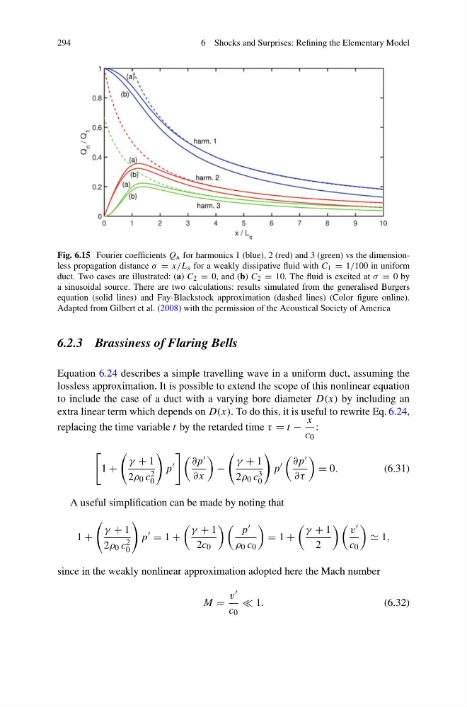
Fig. 6.15 Fourier coefficients Q n for harmonics 1 (blue), 2 (red) and 3 (green) vs the dimensionless propagation distance σ = x/L s for a weakly dissipative fluid with C 1 = 1/100 in uniform
duct. Two cases are illustrated: (a) C 2 = 0, and (b) C 2 = 10. The fluid is excited at σ = 0 by
a sinusoidal source. There are two calculations: results simulated from the generalised Burgers
equation (solid lines) and Fay-Blackstock approximation (dashed lines) (Color figure online).
Adapted from Gilbert et al. (2008) with the permission of the Acoustical Society of America
6.2.3 Brassiness of Flaring Bells
Equation 6.24 describes a simple travelling wave in a uniform duct, assuming the
lossless approximation. It is possible to extend the scope of this nonlinear equation
to include the case of a duct with a varying bore diameter D(x) by including an
extra linear term which depends on D(x). To do this, it is useful to rewrite Eq. 6.24,
replacing the time variable t by the retarded time τ = t −
x
c 0
:
1 +
γ + 1
2ρ 0 c 2
0
p
∂p
∂x
−
γ + 1
2ρ 0 c 3
0
p
∂p
∂τ
= 0.
(6.31)
A useful simplification can be made by noting that
1 +
γ + 1
2ρ 0 c 2
0
p
= 1 +
γ + 1
2c 0
p
ρ 0 c 0
= 1 +
γ + 1
2
v
c 0
1,
since in the weakly nonlinear approximation adopted here the Mach number
M =
v
c 0
1.
(6.32)
6 Shocks and Surprises: Refining the Elementary Model
Fig. 6.15 Fourier coefficients Q n for harmonics 1 (blue), 2 (red) and 3 (green) vs the dimensionless propagation distance σ = x/L s for a weakly dissipative fluid with C 1 = 1/100 in uniform
duct. Two cases are illustrated: (a) C 2 = 0, and (b) C 2 = 10. The fluid is excited at σ = 0 by
a sinusoidal source. There are two calculations: results simulated from the generalised Burgers
equation (solid lines) and Fay-Blackstock approximation (dashed lines) (Color figure online).
Adapted from Gilbert et al. (2008) with the permission of the Acoustical Society of America
6.2.3 Brassiness of Flaring Bells
Equation 6.24 describes a simple travelling wave in a uniform duct, assuming the
lossless approximation. It is possible to extend the scope of this nonlinear equation
to include the case of a duct with a varying bore diameter D(x) by including an
extra linear term which depends on D(x). To do this, it is useful to rewrite Eq. 6.24,
replacing the time variable t by the retarded time τ = t −
x
c 0
:
1 +
γ + 1
2ρ 0 c 2
0
p
∂p
∂x
−
γ + 1
2ρ 0 c 3
0
p
∂p
∂τ
= 0.
(6.31)
A useful simplification can be made by noting that
1 +
γ + 1
2ρ 0 c 2
0
p
= 1 +
γ + 1
2c 0
p
ρ 0 c 0
= 1 +
γ + 1
2
v
c 0
1,
since in the weakly nonlinear approximation adopted here the Mach number
M =
v
c 0
1.
(6.32)