

6.2 Going Further: Nonlinear Propagation
295
Equation 6.31 then becomes
∂p
∂x
−
γ + 1
2ρ o c 3
o
p
∂p
∂τ
= 0.
(6.33)
The flaring expansion of the tube is taken into account by adding to the left-hand
side of Eq. 6.33 the additional term p 1
D
dD
dx
:
∂p
∂x
−
γ + 1
2ρ o c 3
o
p
∂p
∂τ
+ p
1
D
dD
dx
= 0.
(6.34)
Generalised Burgers equations including this extra term have been used (Gilbert
et al. 2008) to simulate the behaviour of weakly nonlinear wave propagation in
nonuniform ducts in periodic regimes. The linear limit of these coupled equations
does not lead exactly to the Webster-Lagrange equation, since the dispersive effect
of the flare is not included in the approximation (Gilbert et al. 2007). This is
equivalent to the assumption that the forward travelling wave is reflected only at the
output plane, with the consequence that the model does not correctly reproduce the
resonance frequencies of a flaring brass instrument (Harrison 2018). It does however
capture the main effects of nonlinear propagation, since the major contribution to
the cumulative distortion of the waveform takes place in the earlier portions of the
bore where the rate of flare is very small. Comparisons between simulations and
measurements are presented in Myers et al. (2012), Campbell et al. (2014b) and
Maugeais and Gilbert (2017).
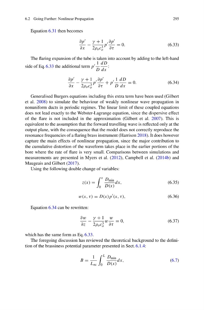
Using the following double change of variables:
z(x) =
x
0
D min
D(x)
dx,
(6.35)
w(x, τ ) = D(x)p
(x, τ ),
(6.36)
Equation 6.34 can be rewritten:
∂w
∂z
−
γ + 1
2ρ o c 3
o
w
w
∂τ
= 0,
(6.37)
which has the same form as Eq. 6.33.
The foregoing discussion has reviewed the theoretical background to the definition of the brassiness potential parameter presented in Sect. 6.1.4:
B =
1
L ec
L
0
D min
D(x)
dx,
(6.7)
295
Equation 6.31 then becomes
∂p
∂x
−
γ + 1
2ρ o c 3
o
p
∂p
∂τ
= 0.
(6.33)
The flaring expansion of the tube is taken into account by adding to the left-hand
side of Eq. 6.33 the additional term p 1
D
dD
dx
:
∂p
∂x
−
γ + 1
2ρ o c 3
o
p
∂p
∂τ
+ p
1
D
dD
dx
= 0.
(6.34)
Generalised Burgers equations including this extra term have been used (Gilbert
et al. 2008) to simulate the behaviour of weakly nonlinear wave propagation in
nonuniform ducts in periodic regimes. The linear limit of these coupled equations
does not lead exactly to the Webster-Lagrange equation, since the dispersive effect
of the flare is not included in the approximation (Gilbert et al. 2007). This is
equivalent to the assumption that the forward travelling wave is reflected only at the
output plane, with the consequence that the model does not correctly reproduce the
resonance frequencies of a flaring brass instrument (Harrison 2018). It does however
capture the main effects of nonlinear propagation, since the major contribution to
the cumulative distortion of the waveform takes place in the earlier portions of the
bore where the rate of flare is very small. Comparisons between simulations and
measurements are presented in Myers et al. (2012), Campbell et al. (2014b) and
Maugeais and Gilbert (2017).
Using the following double change of variables:
z(x) =
x
0
D min
D(x)
dx,
(6.35)
w(x, τ ) = D(x)p
(x, τ ),
(6.36)
Equation 6.34 can be rewritten:
∂w
∂z
−
γ + 1
2ρ o c 3
o
w
w
∂τ
= 0,
(6.37)
which has the same form as Eq. 6.33.
The foregoing discussion has reviewed the theoretical background to the definition of the brassiness potential parameter presented in Sect. 6.1.4:
B =
1
L ec
L
0
D min
D(x)
dx,
(6.7)