

250
5 Blow That Horn: An Elementary Model of Brass Playing
Having found a time domain representation of the third constituent equation of
the elementary model in terms of complex mode parameters, we follow the same
procedure as we used with the real mode representation. The two other equations of
the elementary model, describing the 1DOF lip oscillator (Eq. 5.1) and the volume
flow through the lips (Eq. 5.7), are employed to obtain the following set of secondand first-order ODEs:
⎧
⎪ ⎨
⎪ ⎩
d 2 h(t)
dt 2 = −ω 2
l h(t) −
ω l
q l
dh(t)
dt
−
p(t)
μ
+ ω 2
l h 0 +
p m
μ
dp n
dt
= s n p n (t) + Z c C n
2
ρ wh(t)
√
p m − p(t) for n ∈ [1 : N ],
(5.36)
where as before we assume that at each time t, p m − p(t) > 0 and h(t) > 0.
In the state-space representation (Eq. 5.29), the state vector X has 2(N + 1) real
components defined as follows (see, e.g. Velut et al. (2017a)):
X =
h
dh
dt
Re(p 1 ) ... Re(p N ) Im(p 1 ) ... Im(p N )
T
,
(5.37)
where each complex component p n has been split into its real part Re(p n ) and its
imaginary part Im(p n ).
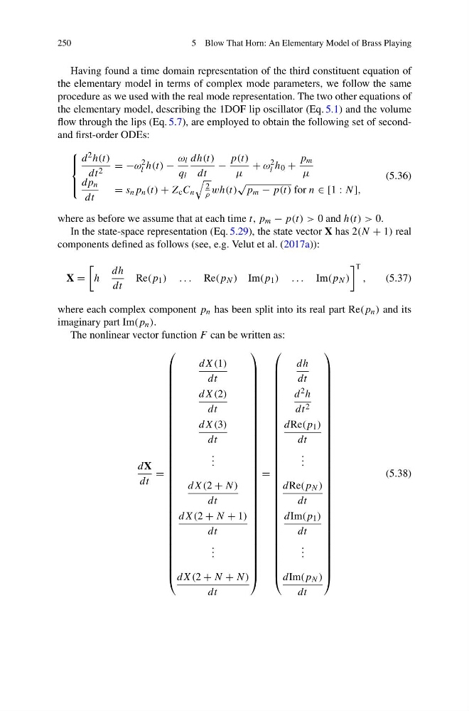
The nonlinear vector function F can be written as:
dX
dt
=
⎛
⎜
⎜
⎜
⎜
⎜
⎜
⎜
⎜
⎜
⎜
⎜
⎜
⎜
⎜
⎜
⎜
⎜
⎜
⎜
⎜
⎜
⎜
⎜
⎜
⎜
⎜
⎜
⎜
⎜
⎜
⎜
⎜
⎝
dX(1)
dt
dX(2)
dt
dX(3)
dt
. . .
dX(2 + N)
dt
dX(2 + N + 1)
dt
. . .
dX(2 + N + N)
dt
⎞
⎟
⎟
⎟
⎟
⎟
⎟
⎟
⎟
⎟
⎟
⎟
⎟
⎟
⎟
⎟
⎟
⎟
⎟
⎟
⎟
⎟
⎟
⎟
⎟
⎟
⎟
⎟
⎟
⎟
⎟
⎟
⎟
⎠
=
⎛
⎜
⎜
⎜
⎜
⎜
⎜
⎜
⎜
⎜
⎜
⎜
⎜
⎜
⎜
⎜
⎜
⎜
⎜
⎜
⎜
⎜
⎜
⎜
⎜
⎜
⎜
⎜
⎜
⎜
⎜
⎜
⎜
⎝
dh
dt
d 2 h
dt 2
dRe(p 1 )
dt
. . .
dRe(p N )
dt
dIm(p 1 )
dt
. . .
dIm(p N )
dt
⎞
⎟
⎟
⎟
⎟
⎟
⎟
⎟
⎟
⎟
⎟
⎟
⎟
⎟
⎟
⎟
⎟
⎟
⎟
⎟
⎟
⎟
⎟
⎟
⎟
⎟
⎟
⎟
⎟
⎟
⎟
⎟
⎟
⎠
(5.38)
5 Blow That Horn: An Elementary Model of Brass Playing
Having found a time domain representation of the third constituent equation of
the elementary model in terms of complex mode parameters, we follow the same
procedure as we used with the real mode representation. The two other equations of
the elementary model, describing the 1DOF lip oscillator (Eq. 5.1) and the volume
flow through the lips (Eq. 5.7), are employed to obtain the following set of secondand first-order ODEs:
⎧
⎪ ⎨
⎪ ⎩
d 2 h(t)
dt 2 = −ω 2
l h(t) −
ω l
q l
dh(t)
dt
−
p(t)
μ
+ ω 2
l h 0 +
p m
μ
dp n
dt
= s n p n (t) + Z c C n
2
ρ wh(t)
√
p m − p(t) for n ∈ [1 : N ],
(5.36)
where as before we assume that at each time t, p m − p(t) > 0 and h(t) > 0.
In the state-space representation (Eq. 5.29), the state vector X has 2(N + 1) real
components defined as follows (see, e.g. Velut et al. (2017a)):
X =
h
dh
dt
Re(p 1 ) ... Re(p N ) Im(p 1 ) ... Im(p N )
T
,
(5.37)
where each complex component p n has been split into its real part Re(p n ) and its
imaginary part Im(p n ).
The nonlinear vector function F can be written as:
dX
dt
=
⎛
⎜
⎜
⎜
⎜
⎜
⎜
⎜
⎜
⎜
⎜
⎜
⎜
⎜
⎜
⎜
⎜
⎜
⎜
⎜
⎜
⎜
⎜
⎜
⎜
⎜
⎜
⎜
⎜
⎜
⎜
⎜
⎜
⎝
dX(1)
dt
dX(2)
dt
dX(3)
dt
. . .
dX(2 + N)
dt
dX(2 + N + 1)
dt
. . .
dX(2 + N + N)
dt
⎞
⎟
⎟
⎟
⎟
⎟
⎟
⎟
⎟
⎟
⎟
⎟
⎟
⎟
⎟
⎟
⎟
⎟
⎟
⎟
⎟
⎟
⎟
⎟
⎟
⎟
⎟
⎟
⎟
⎟
⎟
⎟
⎟
⎠
=
⎛
⎜
⎜
⎜
⎜
⎜
⎜
⎜
⎜
⎜
⎜
⎜
⎜
⎜
⎜
⎜
⎜
⎜
⎜
⎜
⎜
⎜
⎜
⎜
⎜
⎜
⎜
⎜
⎜
⎜
⎜
⎜
⎜
⎝
dh
dt
d 2 h
dt 2
dRe(p 1 )
dt
. . .
dRe(p N )
dt
dIm(p 1 )
dt
. . .
dIm(p N )
dt
⎞
⎟
⎟
⎟
⎟
⎟
⎟
⎟
⎟
⎟
⎟
⎟
⎟
⎟
⎟
⎟
⎟
⎟
⎟
⎟
⎟
⎟
⎟
⎟
⎟
⎟
⎟
⎟
⎟
⎟
⎟
⎟
⎟
⎠
(5.38)