

5.4 Going Further: From Linear Stability Analysis to Oscillation Regimes
251
=
⎛
⎜
⎜
⎜
⎜
⎜
⎜
⎜
⎜
⎜
⎜
⎜
⎜
⎜
⎜
⎜
⎜
⎜
⎜
⎜
⎜
⎜
⎜
⎜
⎜
⎜
⎜
⎜
⎜
⎜
⎜
⎝
X(2)
−ω 2
l X(1) −
ω l
q l
X(2) −
p(t)
μ
+ ω 2
l h 0 +
p m
μ
Re
s 1 (X(3) + jX(2 + N + 1)) + C 1 .Z c .
2
ρ
wX(1)
√
p m − p(t)
. . .
Re
s N (X(2 + N) + jX(2 + N + N)) + C N .Z c .
2
ρ
wX(1)
√
p m − p(t)
Im
s 1 (X(3) + jX(2 + N + 1)) + C 1 .Z c .
2
ρ
wX(1)
√
p m − p(t)
. . .
Im
s N (X(2 + N) + jX(2 + N + N)) + C N .Z c .
2
ρ
wX(1)
√
p m − p(t)
⎞
⎟
⎟
⎟
⎟
⎟
⎟
⎟
⎟
⎟
⎟
⎟
⎟
⎟
⎟
⎟
⎟
⎟
⎟
⎟
⎟
⎟
⎟
⎟
⎟
⎟
⎟
⎟
⎟
⎟
⎟
⎠
,
(5.39)
with
p(t) = 2
N +2
k=3
X(k).
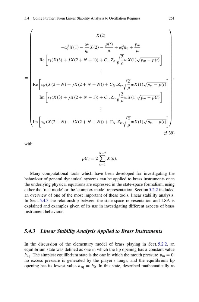
Many computational tools which have been developed for investigating the
behaviour of general dynamical systems can be applied to brass instruments once
the underlying physical equations are expressed in the state-space formalism, using
either the ‘real mode’ or the ‘complex mode’ representation. Section 5.2.2 included
an overview of one of the most important of these tools, linear stability analysis.
In Sect. 5.4.3 the relationship between the state-space representation and LSA is
explained and examples given of its use in investigating different aspects of brass
instrument behaviour.
5.4.3 Linear Stability Analysis Applied to Brass Instruments
In the discussion of the elementary model of brass playing in Sect. 5.2.2, an
equilibrium state was defined as one in which the lip opening has a constant value
h eq . The simplest equilibrium state is the one in which the mouth pressure p m = 0:
no excess pressure is generated by the player’s lungs, and the equilibrium lip
opening has its lowest value h eq = h 0 . In this state, described mathematically as
251
=
⎛
⎜
⎜
⎜
⎜
⎜
⎜
⎜
⎜
⎜
⎜
⎜
⎜
⎜
⎜
⎜
⎜
⎜
⎜
⎜
⎜
⎜
⎜
⎜
⎜
⎜
⎜
⎜
⎜
⎜
⎜
⎝
X(2)
−ω 2
l X(1) −
ω l
q l
X(2) −
p(t)
μ
+ ω 2
l h 0 +
p m
μ
Re
s 1 (X(3) + jX(2 + N + 1)) + C 1 .Z c .
2
ρ
wX(1)
√
p m − p(t)
. . .
Re
s N (X(2 + N) + jX(2 + N + N)) + C N .Z c .
2
ρ
wX(1)
√
p m − p(t)
Im
s 1 (X(3) + jX(2 + N + 1)) + C 1 .Z c .
2
ρ
wX(1)
√
p m − p(t)
. . .
Im
s N (X(2 + N) + jX(2 + N + N)) + C N .Z c .
2
ρ
wX(1)
√
p m − p(t)
⎞
⎟
⎟
⎟
⎟
⎟
⎟
⎟
⎟
⎟
⎟
⎟
⎟
⎟
⎟
⎟
⎟
⎟
⎟
⎟
⎟
⎟
⎟
⎟
⎟
⎟
⎟
⎟
⎟
⎟
⎟
⎠
,
(5.39)
with
p(t) = 2
N +2
k=3
X(k).
Many computational tools which have been developed for investigating the
behaviour of general dynamical systems can be applied to brass instruments once
the underlying physical equations are expressed in the state-space formalism, using
either the ‘real mode’ or the ‘complex mode’ representation. Section 5.2.2 included
an overview of one of the most important of these tools, linear stability analysis.
In Sect. 5.4.3 the relationship between the state-space representation and LSA is
explained and examples given of its use in investigating different aspects of brass
instrument behaviour.
5.4.3 Linear Stability Analysis Applied to Brass Instruments
In the discussion of the elementary model of brass playing in Sect. 5.2.2, an
equilibrium state was defined as one in which the lip opening has a constant value
h eq . The simplest equilibrium state is the one in which the mouth pressure p m = 0:
no excess pressure is generated by the player’s lungs, and the equilibrium lip
opening has its lowest value h eq = h 0 . In this state, described mathematically as