

5.4 Going Further: From Linear Stability Analysis to Oscillation Regimes
243
reformulation of the brass model in Sect. 5.4.2, we illustrate the procedure by
reformulating the simpler system of the Van der Pol self-sustained oscillator as a
dynamical system of dimension 2. We begin by defining a state vector X, with the
following components:
⎡
⎣
X 1 = p(t)
X 2 =
dp(t)
dt
⎤
⎦ .
(5.17)
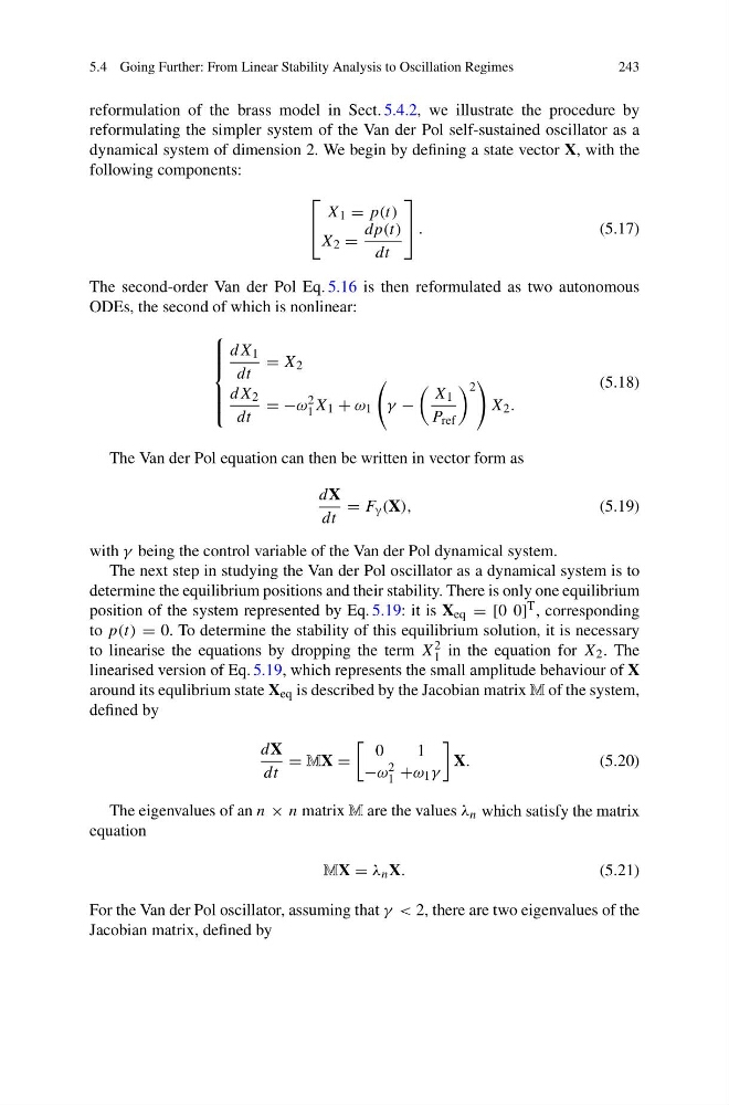
The second-order Van der Pol Eq. 5.16 is then reformulated as two autonomous
ODEs, the second of which is nonlinear:
⎧
⎪ ⎪ ⎪ ⎨
⎪ ⎪ ⎪ ⎩
dX 1
dt
= X 2
dX 2
dt
= −ω 2
1 X 1 + ω 1
γ −
X 1
P ref
2
X 2 .
(5.18)
The Van der Pol equation can then be written in vector form as
dX
dt
= F γ (X),
(5.19)
with γ being the control variable of the Van der Pol dynamical system.
The next step in studying the Van der Pol oscillator as a dynamical system is to
determine the equilibrium positions and their stability. There is only one equilibrium
position of the system represented by Eq. 5.19: it is X eq = [0 0] T , corresponding
to p(t) = 0. To determine the stability of this equilibrium solution, it is necessary
to linearise the equations by dropping the term X 2
1 in the equation for X 2 . The
linearised version of Eq. 5.19, which represents the small amplitude behaviour of X
around its equlibrium state X eq is described by the Jacobian matrix M of the system,
defined by
dX
dt
= MX =
0
1
−ω 2
1 +ω 1 γ
X.
(5.20)
The eigenvalues of an n × n matrix M are the values λ n which satisfy the matrix
equation
MX = λ n X.
(5.21)
For the Van der Pol oscillator, assuming that γ < 2, there are two eigenvalues of the
Jacobian matrix, defined by
243
reformulation of the brass model in Sect. 5.4.2, we illustrate the procedure by
reformulating the simpler system of the Van der Pol self-sustained oscillator as a
dynamical system of dimension 2. We begin by defining a state vector X, with the
following components:
⎡
⎣
X 1 = p(t)
X 2 =
dp(t)
dt
⎤
⎦ .
(5.17)
The second-order Van der Pol Eq. 5.16 is then reformulated as two autonomous
ODEs, the second of which is nonlinear:
⎧
⎪ ⎪ ⎪ ⎨
⎪ ⎪ ⎪ ⎩
dX 1
dt
= X 2
dX 2
dt
= −ω 2
1 X 1 + ω 1
γ −
X 1
P ref
2
X 2 .
(5.18)
The Van der Pol equation can then be written in vector form as
dX
dt
= F γ (X),
(5.19)
with γ being the control variable of the Van der Pol dynamical system.
The next step in studying the Van der Pol oscillator as a dynamical system is to
determine the equilibrium positions and their stability. There is only one equilibrium
position of the system represented by Eq. 5.19: it is X eq = [0 0] T , corresponding
to p(t) = 0. To determine the stability of this equilibrium solution, it is necessary
to linearise the equations by dropping the term X 2
1 in the equation for X 2 . The
linearised version of Eq. 5.19, which represents the small amplitude behaviour of X
around its equlibrium state X eq is described by the Jacobian matrix M of the system,
defined by
dX
dt
= MX =
0
1
−ω 2
1 +ω 1 γ
X.
(5.20)
The eigenvalues of an n × n matrix M are the values λ n which satisfy the matrix
equation
MX = λ n X.
(5.21)
For the Van der Pol oscillator, assuming that γ < 2, there are two eigenvalues of the
Jacobian matrix, defined by