

4.7 Going Further: Calculating Input Impedance
205
= α + j
ω
v p
ω
c
1.045 r
−1
v + j
1 + r
−1
v
.
(4.109)
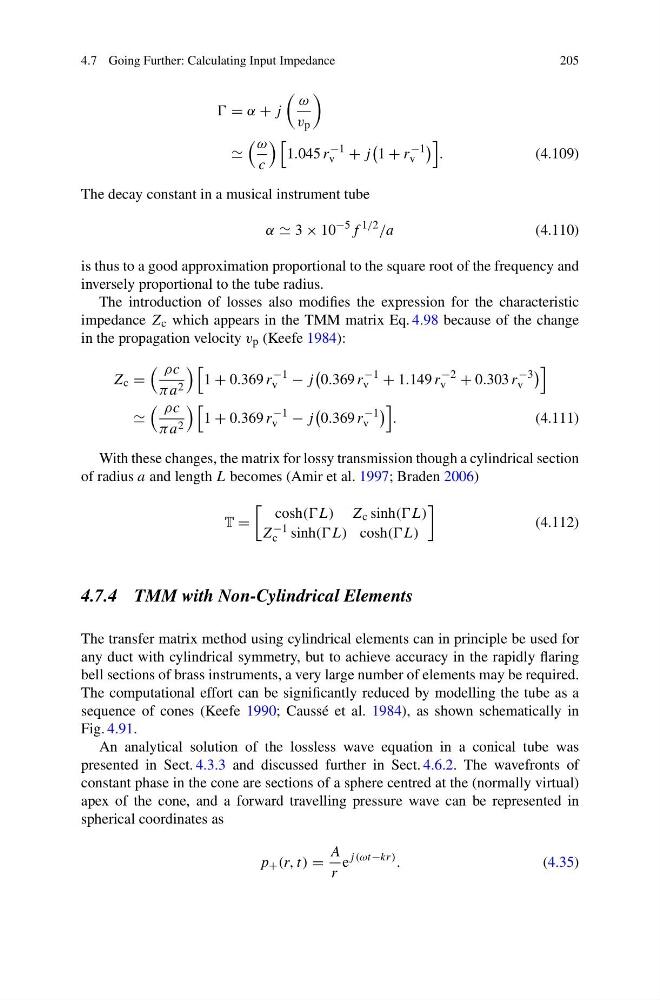
The decay constant in a musical instrument tube
α 3 × 10
−5 f
1/2 /a
(4.110)
is thus to a good approximation proportional to the square root of the frequency and
inversely proportional to the tube radius.
The introduction of losses also modifies the expression for the characteristic
impedance Z c which appears in the TMM matrix Eq. 4.98 because of the change
in the propagation velocity v p (Keefe 1984):
Z c =
ρc
πa 2
1 + 0.369 r
−1
v − j
0.369 r
−1
v + 1.149 r
−2
v + 0.303 r
−3
v
ρc
πa 2
1 + 0.369 r
−1
v − j
0.369 r
−1
v
.
(4.111)
With these changes, the matrix for lossy transmission though a cylindrical section
of radius a and length L becomes (Amir et al. 1997; Braden 2006)
T =
cosh((L) Z c sinh((L)
Z −1
c sinh((L) cosh((L)
(4.112)
4.7.4 TMM with Non-Cylindrical Elements
The transfer matrix method using cylindrical elements can in principle be used for
any duct with cylindrical symmetry, but to achieve accuracy in the rapidly flaring
bell sections of brass instruments, a very large number of elements may be required.
The computational effort can be significantly reduced by modelling the tube as a
sequence of cones (Keefe 1990; Caussé et al. 1984), as shown schematically in
Fig. 4.91.
An analytical solution of the lossless wave equation in a conical tube was
presented in Sect. 4.3.3 and discussed further in Sect. 4.6.2. The wavefronts of
constant phase in the cone are sections of a sphere centred at the (normally virtual)
apex of the cone, and a forward travelling pressure wave can be represented in
spherical coordinates as
p + (r, t) =
A
r
e
j (ωt−kr) .
(4.35)
205
= α + j
ω
v p
ω
c
1.045 r
−1
v + j
1 + r
−1
v
.
(4.109)
The decay constant in a musical instrument tube
α 3 × 10
−5 f
1/2 /a
(4.110)
is thus to a good approximation proportional to the square root of the frequency and
inversely proportional to the tube radius.
The introduction of losses also modifies the expression for the characteristic
impedance Z c which appears in the TMM matrix Eq. 4.98 because of the change
in the propagation velocity v p (Keefe 1984):
Z c =
ρc
πa 2
1 + 0.369 r
−1
v − j
0.369 r
−1
v + 1.149 r
−2
v + 0.303 r
−3
v
ρc
πa 2
1 + 0.369 r
−1
v − j
0.369 r
−1
v
.
(4.111)
With these changes, the matrix for lossy transmission though a cylindrical section
of radius a and length L becomes (Amir et al. 1997; Braden 2006)
T =
cosh((L) Z c sinh((L)
Z −1
c sinh((L) cosh((L)
(4.112)
4.7.4 TMM with Non-Cylindrical Elements
The transfer matrix method using cylindrical elements can in principle be used for
any duct with cylindrical symmetry, but to achieve accuracy in the rapidly flaring
bell sections of brass instruments, a very large number of elements may be required.
The computational effort can be significantly reduced by modelling the tube as a
sequence of cones (Keefe 1990; Caussé et al. 1984), as shown schematically in
Fig. 4.91.
An analytical solution of the lossless wave equation in a conical tube was
presented in Sect. 4.3.3 and discussed further in Sect. 4.6.2. The wavefronts of
constant phase in the cone are sections of a sphere centred at the (normally virtual)
apex of the cone, and a forward travelling pressure wave can be represented in
spherical coordinates as
p + (r, t) =
A
r
e
j (ωt−kr) .
(4.35)