

10 PHSD—A Microscopic Transport Approach for Strongly Interacting Systems
127
time [33] without introducing any new parameter in the PHSD approach since the
electromagnetic coupling is well known.
Numerical tests of the parton dynamics with respect to conservation laws, interaction rates in and out-off equilibrium in a finite box with periodic boundary conditions
have been presented in [39]. In fact, in [39] it was shown that the PHSD calculations
in the box give practically the same results in equilibrium as the DQPM. We note
in passing that the total energy is conserved in the box calculations up to about 3
digits while in the heavy-ion collisions addressed here in the following the violation
of energy conservation is typically less than 1% [34].
10.3 Transport Properties of the Partonic System
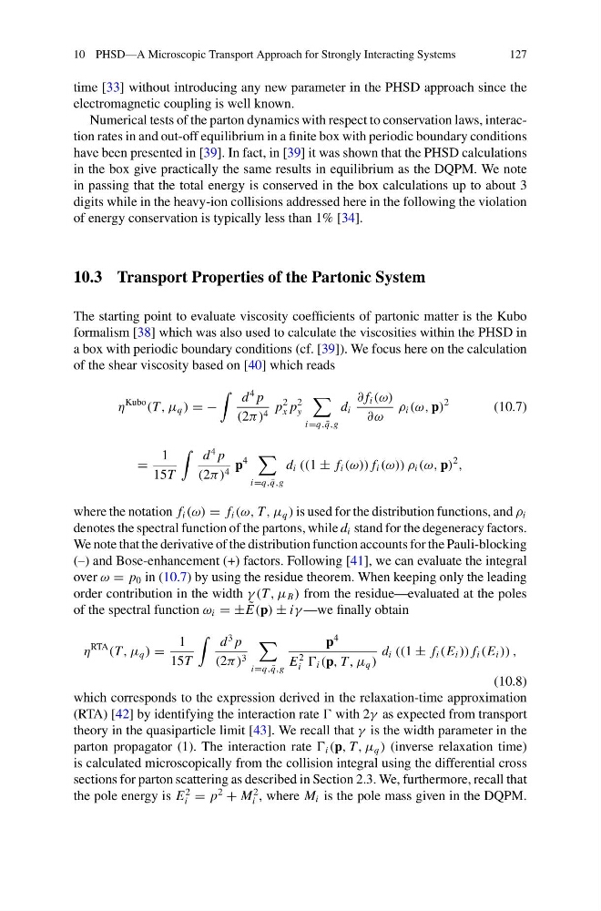
The starting point to evaluate viscosity coefficients of partonic matter is the Kubo
formalism [38] which was also used to calculate the viscosities within the PHSD in
a box with periodic boundary conditions (cf. [39]). We focus here on the calculation
of the shear viscosity based on [40] which reads
η
Kubo
(T, μ q ) = −
d
4 p
(2π) 4 p
2
x p
2
y
i=q, ¯
q,g
d i
∂ f i (ω)
∂ω
ρ i (ω, p)
2
(10.7)
=
1
15T
d
4 p
(2π) 4 p
4
i=q, ¯
q,g
d i ((1 ± f i (ω)) f i (ω)) ρ i (ω, p)
2
,
where the notation f i (ω) = f i (ω, T, μ q ) is used for the distribution functions, and ρ i
denotes the spectral function of the partons, while d i stand for the degeneracy factors.
We note that the derivative of the distribution function accounts for the Pauli-blocking
(–) and Bose-enhancement (+) factors. Following [41], we can evaluate the integral
over ω = p 0 in (10.7) by using the residue theorem. When keeping only the leading
order contribution in the width γ (T, μ B ) from the residue—evaluated at the poles
of the spectral function ω i = ± ˜
E(p) ± iγ —we finally obtain
η
RTA
(T, μ q ) =
1
15T
d
3 p
(2π) 3
i=q, ¯
q,g
p
4
E
2
i i (p, T, μ q )
d i ((1 ± f i (E i )) f i (E i )) ,
(10.8)
which corresponds to the expression derived in the relaxation-time approximation
(RTA) [42] by identifying the interaction rate with 2γ as expected from transport
theory in the quasiparticle limit [43]. We recall that γ is the width parameter in the
parton propagator (1). The interaction rate i (p, T, μ q ) (inverse relaxation time)
is calculated microscopically from the collision integral using the differential cross
sections for parton scattering as described in Section 2.3. We, furthermore, recall that
the pole energy is E
2
i = p
2
+ M
2
i , where M i is the pole mass given in the DQPM.
127
time [33] without introducing any new parameter in the PHSD approach since the
electromagnetic coupling is well known.
Numerical tests of the parton dynamics with respect to conservation laws, interaction rates in and out-off equilibrium in a finite box with periodic boundary conditions
have been presented in [39]. In fact, in [39] it was shown that the PHSD calculations
in the box give practically the same results in equilibrium as the DQPM. We note
in passing that the total energy is conserved in the box calculations up to about 3
digits while in the heavy-ion collisions addressed here in the following the violation
of energy conservation is typically less than 1% [34].
10.3 Transport Properties of the Partonic System
The starting point to evaluate viscosity coefficients of partonic matter is the Kubo
formalism [38] which was also used to calculate the viscosities within the PHSD in
a box with periodic boundary conditions (cf. [39]). We focus here on the calculation
of the shear viscosity based on [40] which reads
η
Kubo
(T, μ q ) = −
d
4 p
(2π) 4 p
2
x p
2
y
i=q, ¯
q,g
d i
∂ f i (ω)
∂ω
ρ i (ω, p)
2
(10.7)
=
1
15T
d
4 p
(2π) 4 p
4
i=q, ¯
q,g
d i ((1 ± f i (ω)) f i (ω)) ρ i (ω, p)
2
,
where the notation f i (ω) = f i (ω, T, μ q ) is used for the distribution functions, and ρ i
denotes the spectral function of the partons, while d i stand for the degeneracy factors.
We note that the derivative of the distribution function accounts for the Pauli-blocking
(–) and Bose-enhancement (+) factors. Following [41], we can evaluate the integral
over ω = p 0 in (10.7) by using the residue theorem. When keeping only the leading
order contribution in the width γ (T, μ B ) from the residue—evaluated at the poles
of the spectral function ω i = ± ˜
E(p) ± iγ —we finally obtain
η
RTA
(T, μ q ) =
1
15T
d
3 p
(2π) 3
i=q, ¯
q,g
p
4
E
2
i i (p, T, μ q )
d i ((1 ± f i (E i )) f i (E i )) ,
(10.8)
which corresponds to the expression derived in the relaxation-time approximation
(RTA) [42] by identifying the interaction rate with 2γ as expected from transport
theory in the quasiparticle limit [43]. We recall that γ is the width parameter in the
parton propagator (1). The interaction rate i (p, T, μ q ) (inverse relaxation time)
is calculated microscopically from the collision integral using the differential cross
sections for parton scattering as described in Section 2.3. We, furthermore, recall that
the pole energy is E
2
i = p
2
+ M
2
i , where M i is the pole mass given in the DQPM.