

446
13 Metrology Technology of Lunar Lander
of position parameters of the whole metrology network was t = 3q + 6m + 6n + 6p, and
the total number of observation equations was n = 3mq +2nq +2C
2
n +4np+ p. In the
adjustment calculation, the three translation and rotation parameters of the first station
are all 0 in the measurement coordinate system of the first station, and the whole
metrology network should meet n ≥ t−6. Then it could be solved according to the
principle of least squares. In the whole metrology network, the error equation could
be classified into four types: the azimuth error equation, the zenith error equation, the
slant range error equation and the reference length constraint condition equation. The
translation and rotation parameters of station i relative to the measuring coordinate
system were (X 0i , Y 0i , Z 0i , R xi , R yi , R zi ), and the coordinates of the orientation point
k in the coordinate system of station I were (X ik , Y ik , Z ik ), and the coordinates in
the measurement coordinate system were (X k , Y k , Z k ). When the angle, distance and
mutual aiming value were applied to formulate the error equation, it was necessary to
transform directional point k from the station i coordinate system to the measurement
coordinate system [9].
⎡
⎣
X ik
Y ik
Z ik
⎤
⎦ =
⎡
⎣
a i1 b i1 c i1
a i2 b i2 c i2
a i3 b i3 c i3
⎤
⎦ ·
⎡
⎣
X k − X 0i
Y k − Y 0i
Z k − Z 0i
⎤
⎦
(13.3)
3. Analysis of Accuracy
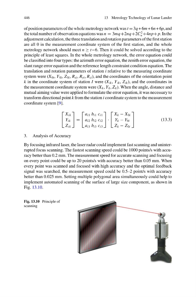
By focusing infrared laser, the laser radar could implement fast scanning and uninterrupted focus scanning. The fastest scanning speed could be 1000 points/s with accuracy better than 0.2 mm. The measurement speed for accurate scanning and focusing
on every point could be up to 20 points/s with accuracy better than 0.05 mm. When
every point was scanned and focused with high accuracy and the optimal feedback
signal was searched, the measurement speed could be 0.5–2 point/s with accuracy
better than 0.025 mm. Setting multiple polygonal area simultaneously could help to
implement automated scanning of the surface of large size component, as shown in
Fig. 13.10.
Fig. 13.10 Principle of
scanning
13 Metrology Technology of Lunar Lander
of position parameters of the whole metrology network was t = 3q + 6m + 6n + 6p, and
the total number of observation equations was n = 3mq +2nq +2C
2
n +4np+ p. In the
adjustment calculation, the three translation and rotation parameters of the first station
are all 0 in the measurement coordinate system of the first station, and the whole
metrology network should meet n ≥ t−6. Then it could be solved according to the
principle of least squares. In the whole metrology network, the error equation could
be classified into four types: the azimuth error equation, the zenith error equation, the
slant range error equation and the reference length constraint condition equation. The
translation and rotation parameters of station i relative to the measuring coordinate
system were (X 0i , Y 0i , Z 0i , R xi , R yi , R zi ), and the coordinates of the orientation point
k in the coordinate system of station I were (X ik , Y ik , Z ik ), and the coordinates in
the measurement coordinate system were (X k , Y k , Z k ). When the angle, distance and
mutual aiming value were applied to formulate the error equation, it was necessary to
transform directional point k from the station i coordinate system to the measurement
coordinate system [9].
⎡
⎣
X ik
Y ik
Z ik
⎤
⎦ =
⎡
⎣
a i1 b i1 c i1
a i2 b i2 c i2
a i3 b i3 c i3
⎤
⎦ ·
⎡
⎣
X k − X 0i
Y k − Y 0i
Z k − Z 0i
⎤
⎦
(13.3)
3. Analysis of Accuracy
By focusing infrared laser, the laser radar could implement fast scanning and uninterrupted focus scanning. The fastest scanning speed could be 1000 points/s with accuracy better than 0.2 mm. The measurement speed for accurate scanning and focusing
on every point could be up to 20 points/s with accuracy better than 0.05 mm. When
every point was scanned and focused with high accuracy and the optimal feedback
signal was searched, the measurement speed could be 0.5–2 point/s with accuracy
better than 0.025 mm. Setting multiple polygonal area simultaneously could help to
implement automated scanning of the surface of large size component, as shown in
Fig. 13.10.
Fig. 13.10 Principle of
scanning