

5 Phase-Field-Crystal Model: A Tool for Probing Atoms in TSV
127
new domain for filler materials in the near future [42]. In this section, simulating the
graphene structure through the PFC models will be presented in brief.
To simulate solid phases with more complex structures, higher order of correlation
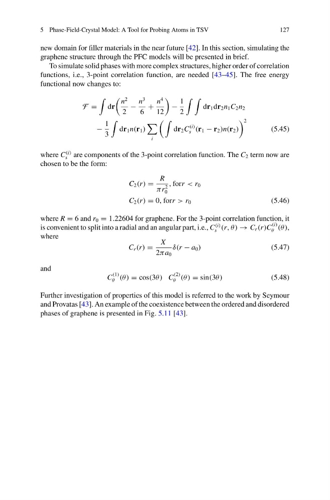
functions, i.e., 3-point correlation function, are needed [43–45]. The free energy
functional now changes to:
F =
dr
n
2
2
−
n
3
6
+
n
4
12
−
1
2
dr 1 dr 2 n 1 C 2 n 2
−
1
3
dr 1 n(r 1 )
i
dr 2 C
(i)
s (r 1 − r 2 )n(r 2 )
2
(5.45)
where C
(i)
s are components of the 3-point correlation function. The C 2 term now are
chosen to be the form:
C 2 (r) =
R
π r
2
0
, forr < r 0
C 2 (r) = 0, forr > r 0
(5.46)
where R = 6 and r 0 = 1.22604 for graphene. For the 3-point correlation function, it
is convenient to split into a radial and an angular part, i.e., C
(i)
s (r, θ) → C r (r)C
(i)
θ (θ ),
where
C r (r) =
X
2π a 0
δ(r − a 0 )
(5.47)
and
C
(1)
θ (θ ) = cos(3θ) C
(2)
θ (θ ) = sin(3θ)
(5.48)
Further investigation of properties of this model is referred to the work by Seymour
and Provatas [43]. An example of the coexistence between the ordered and disordered
phases of graphene is presented in Fig. 5.11 [43].
127
new domain for filler materials in the near future [42]. In this section, simulating the
graphene structure through the PFC models will be presented in brief.
To simulate solid phases with more complex structures, higher order of correlation
functions, i.e., 3-point correlation function, are needed [43–45]. The free energy
functional now changes to:
F =
dr
n
2
2
−
n
3
6
+
n
4
12
−
1
2
dr 1 dr 2 n 1 C 2 n 2
−
1
3
dr 1 n(r 1 )
i
dr 2 C
(i)
s (r 1 − r 2 )n(r 2 )
2
(5.45)
where C
(i)
s are components of the 3-point correlation function. The C 2 term now are
chosen to be the form:
C 2 (r) =
R
π r
2
0
, forr < r 0
C 2 (r) = 0, forr > r 0
(5.46)
where R = 6 and r 0 = 1.22604 for graphene. For the 3-point correlation function, it
is convenient to split into a radial and an angular part, i.e., C
(i)
s (r, θ) → C r (r)C
(i)
θ (θ ),
where
C r (r) =
X
2π a 0
δ(r − a 0 )
(5.47)
and
C
(1)
θ (θ ) = cos(3θ) C
(2)
θ (θ ) = sin(3θ)
(5.48)
Further investigation of properties of this model is referred to the work by Seymour
and Provatas [43]. An example of the coexistence between the ordered and disordered
phases of graphene is presented in Fig. 5.11 [43].