

126
J. Liu et al.
where Q = |K 2 |/|K 1 | =
√
2 is the ratio of the magnitude of the two wave vectors.
In addition, r ∝ (T − T m )/T m is the scaling temperature, where T is the absolute
temperature with unit of Kelvin and T m is the melting temperature. The parameters
in this case are more complicated than that in the one-mode PFC model, and a
Mathematica code Ch5MC2 is given instead:
Mathematica Code (Ch5MC2)
(*free energy functional for square lattice*)
n = n0 + A*(Exp[I*q*{1, 0}.{x, y}] + Exp[I*q*{-1, 0}.{x, y}]
+ Exp[I*q*{0, 1}.{x, y}] + Exp[I*q*{0, -1}.{x, y}]) +
B*(Exp[I*q*{1, 1}.{x, y}] + Exp[I*q*{-1, 1}.{x, y}] +
Exp[I*q*{1, -1}.{x, y}] + Exp[I*q*{-1, -1}.{x, y}]);
n = Collect[TrigExpand[ExpToTrig[n]], 2*A, Simplify]
Ln2 = Laplacian[n, {x, y}];
Ln4 = Laplacian[Ln2, {x, y}];
Ln6 = Laplacian[Ln4, {x, y}];
Ln8 = Laplacian[Ln6, {x, y}];
f = n/2*(-epsilon + 4)*n + n/2*(12*Ln2 + 13*Ln4 + 6*Ln6 + Ln8)
+ nˆ4/4;
intef1 = Integrate[
Collect[f, {A, B}, Simplify], {x, -2 Pi/q, 2 Pi/q},
{y, -2 Pi/q, 2 Pi/q}]/(4 Pi/q)ˆ2;
intef = Expand[intef1]
Solve[D[intef, q] == 0, q]
(*parameters A and B*)
q = 1;
fs = intef
fl = -(epsilon - 4) nlˆ2/2 + nlˆ4/4
dfsA = D[fs, A];
dfsB = D[fs, B];
Solve[{dfsA == 0, dfsB == 0}, {A, B}];
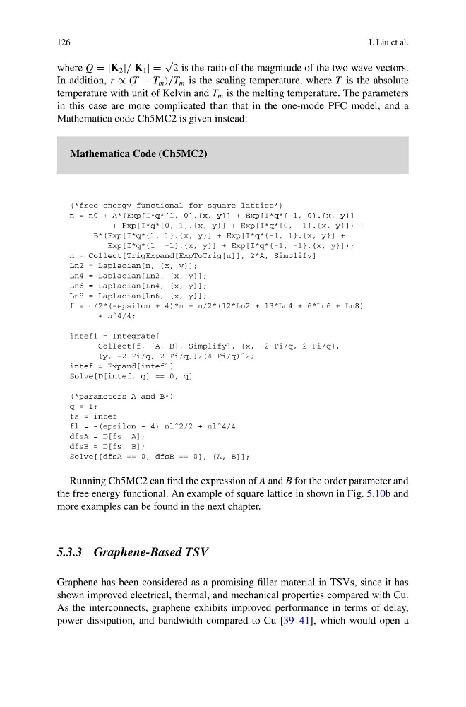
Running Ch5MC2 can find the expression of A and B for the order parameter and
the free energy functional. An example of square lattice in shown in Fig. 5.10b and
more examples can be found in the next chapter.
5.3.3 Graphene-Based TSV
Graphene has been considered as a promising filler material in TSVs, since it has
shown improved electrical, thermal, and mechanical properties compared with Cu.
As the interconnects, graphene exhibits improved performance in terms of delay,
power dissipation, and bandwidth compared to Cu [39–41], which would open a
J. Liu et al.
where Q = |K 2 |/|K 1 | =
√
2 is the ratio of the magnitude of the two wave vectors.
In addition, r ∝ (T − T m )/T m is the scaling temperature, where T is the absolute
temperature with unit of Kelvin and T m is the melting temperature. The parameters
in this case are more complicated than that in the one-mode PFC model, and a
Mathematica code Ch5MC2 is given instead:
Mathematica Code (Ch5MC2)
(*free energy functional for square lattice*)
n = n0 + A*(Exp[I*q*{1, 0}.{x, y}] + Exp[I*q*{-1, 0}.{x, y}]
+ Exp[I*q*{0, 1}.{x, y}] + Exp[I*q*{0, -1}.{x, y}]) +
B*(Exp[I*q*{1, 1}.{x, y}] + Exp[I*q*{-1, 1}.{x, y}] +
Exp[I*q*{1, -1}.{x, y}] + Exp[I*q*{-1, -1}.{x, y}]);
n = Collect[TrigExpand[ExpToTrig[n]], 2*A, Simplify]
Ln2 = Laplacian[n, {x, y}];
Ln4 = Laplacian[Ln2, {x, y}];
Ln6 = Laplacian[Ln4, {x, y}];
Ln8 = Laplacian[Ln6, {x, y}];
f = n/2*(-epsilon + 4)*n + n/2*(12*Ln2 + 13*Ln4 + 6*Ln6 + Ln8)
+ nˆ4/4;
intef1 = Integrate[
Collect[f, {A, B}, Simplify], {x, -2 Pi/q, 2 Pi/q},
{y, -2 Pi/q, 2 Pi/q}]/(4 Pi/q)ˆ2;
intef = Expand[intef1]
Solve[D[intef, q] == 0, q]
(*parameters A and B*)
q = 1;
fs = intef
fl = -(epsilon - 4) nlˆ2/2 + nlˆ4/4
dfsA = D[fs, A];
dfsB = D[fs, B];
Solve[{dfsA == 0, dfsB == 0}, {A, B}];
Running Ch5MC2 can find the expression of A and B for the order parameter and
the free energy functional. An example of square lattice in shown in Fig. 5.10b and
more examples can be found in the next chapter.
5.3.3 Graphene-Based TSV
Graphene has been considered as a promising filler material in TSVs, since it has
shown improved electrical, thermal, and mechanical properties compared with Cu.
As the interconnects, graphene exhibits improved performance in terms of delay,
power dissipation, and bandwidth compared to Cu [39–41], which would open a