

1 KLT, A New Algorithm For SETI
3
• minimizes the total entropy of the sequence
• very good S/N sensibility ad de-noising.
on the other hand, there’s also big disadvantages:
• no fast algorithms exist
• heavy computational task
• no fixed basis a priori but generated each time for each observation.
1.2.2 Eigenvalue Decomposition
Several main topics of research like pattern recognition, financial statistics and many
more have no request about responsiveness, but in other fields like medical, radar and
so on, the time to have the result of a computation is needed almost in real-time. This
is the case of radio astronomy where a natural phenomena has a very short impulse.
A fast Fourier Transform algorithm exists, but not for the KLT: this is the main
issue why it is not so widely used. Nowadays, computer hardwares, equipped with
GPU systems that are dedicated to parallel computing, have solved many complex
scientific tasks and the KLT could take benefit of this new architectures. In digital
signal processing, often, the more the sampled observation is processed the more the
analysis is accurate, however this disagree with the request for real-time. In order
to extract more eigenpairs (eigenvalues and eigenvectors) as possible, the “Krylov
subspace projection methods” are taken in account: Lanczos and Arnoldi are two
well known methods of this type (see [4]). The Arnoldi-algorithm is the selected
one and it return as a result of the computations a set of eigenvectors obtained by an
iterative projection on a given matrix A. The subspace generated from this projection
is called Krilov subspace and the iterations for this method are given by the following
equations:
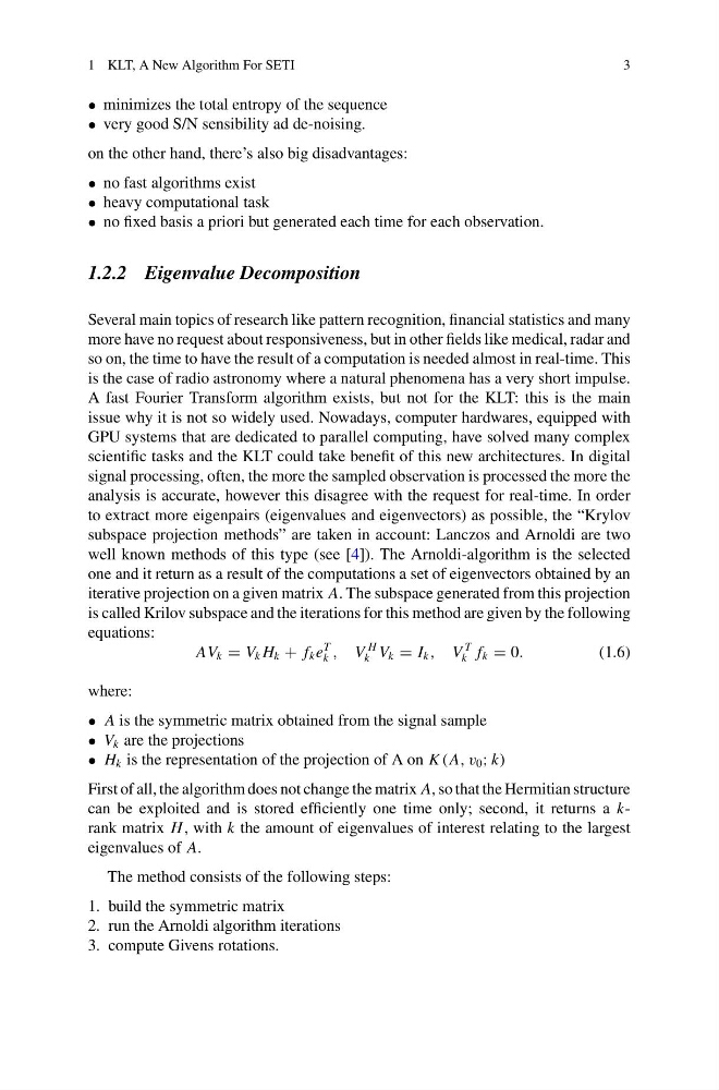
AV k = V k H k + f k e
T
k , V
H
k V k = I k , V
T
k f k = 0.
(1.6)
where:
• A is the symmetric matrix obtained from the signal sample
• V k are the projections
• H k is the representation of the projection of A on K (A, v 0 ; k)
First of all, the algorithm does not change the matrix A, so that the Hermitian structure
can be exploited and is stored efficiently one time only; second, it returns a krank matrix H , with k the amount of eigenvalues of interest relating to the largest
eigenvalues of A.
The method consists of the following steps:
1. build the symmetric matrix
2. run the Arnoldi algorithm iterations
3. compute Givens rotations.
3
• minimizes the total entropy of the sequence
• very good S/N sensibility ad de-noising.
on the other hand, there’s also big disadvantages:
• no fast algorithms exist
• heavy computational task
• no fixed basis a priori but generated each time for each observation.
1.2.2 Eigenvalue Decomposition
Several main topics of research like pattern recognition, financial statistics and many
more have no request about responsiveness, but in other fields like medical, radar and
so on, the time to have the result of a computation is needed almost in real-time. This
is the case of radio astronomy where a natural phenomena has a very short impulse.
A fast Fourier Transform algorithm exists, but not for the KLT: this is the main
issue why it is not so widely used. Nowadays, computer hardwares, equipped with
GPU systems that are dedicated to parallel computing, have solved many complex
scientific tasks and the KLT could take benefit of this new architectures. In digital
signal processing, often, the more the sampled observation is processed the more the
analysis is accurate, however this disagree with the request for real-time. In order
to extract more eigenpairs (eigenvalues and eigenvectors) as possible, the “Krylov
subspace projection methods” are taken in account: Lanczos and Arnoldi are two
well known methods of this type (see [4]). The Arnoldi-algorithm is the selected
one and it return as a result of the computations a set of eigenvectors obtained by an
iterative projection on a given matrix A. The subspace generated from this projection
is called Krilov subspace and the iterations for this method are given by the following
equations:
AV k = V k H k + f k e
T
k , V
H
k V k = I k , V
T
k f k = 0.
(1.6)
where:
• A is the symmetric matrix obtained from the signal sample
• V k are the projections
• H k is the representation of the projection of A on K (A, v 0 ; k)
First of all, the algorithm does not change the matrix A, so that the Hermitian structure
can be exploited and is stored efficiently one time only; second, it returns a krank matrix H , with k the amount of eigenvalues of interest relating to the largest
eigenvalues of A.
The method consists of the following steps:
1. build the symmetric matrix
2. run the Arnoldi algorithm iterations
3. compute Givens rotations.