

4
N. Antonietti and P. Pari
Algorithm 1: Arnoldi first step algorithm
Input: (A,v 0 )
Output:(V k , H k , f k ) such that AV k = V k H k + f k e T
k , V T
k V k = I k and V T
k f k = 0
1. v ← v 1 / v 1
2. w ← Av;
3. H 1 = (α 1 ); V 1 = (v 1 ); f 1 = w − v 1 α 1 ;
4. for j=1,2,3,...,k-1
4.1 β j = f ; v j+1 = f /β j ;
4.2 V j+1 = (V j , v j+1 ); H j =
H j
β j e T
j
4.3 z = Av j+1 ;
4.4 h = V H
j+1 z; H j+1 = (H j , h);
4.5 f j = z − V j+1 h;
5. end
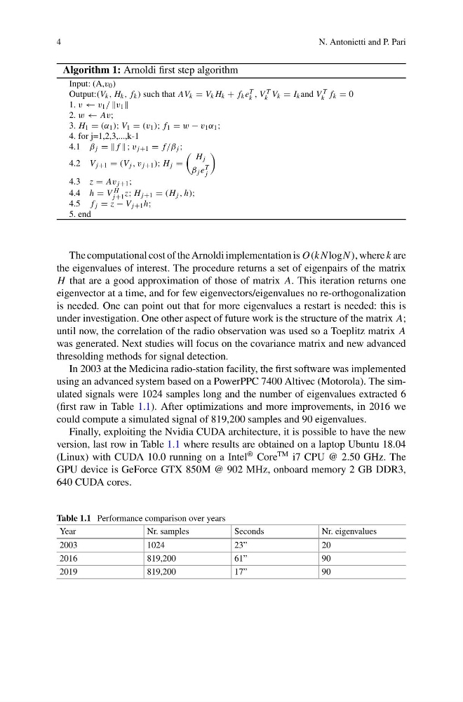
The computational cost of the Arnoldi implementation is O(k N logN ), where k are
the eigenvalues of interest. The procedure returns a set of eigenpairs of the matrix
H that are a good approximation of those of matrix A. This iteration returns one
eigenvector at a time, and for few eigenvectors/eigenvalues no re-orthogonalization
is needed. One can point out that for more eigenvalues a restart is needed: this is
under investigation. One other aspect of future work is the structure of the matrix A;
until now, the correlation of the radio observation was used so a Toeplitz matrix A
was generated. Next studies will focus on the covariance matrix and new advanced
thresolding methods for signal detection.
In 2003 at the Medicina radio-station facility, the first software was implemented
using an advanced system based on a PowerPPC 7400 Altivec (Motorola). The simulated signals were 1024 samples long and the number of eigenvalues extracted 6
(first raw in Table 1.1). After optimizations and more improvements, in 2016 we
could compute a simulated signal of 819,200 samples and 90 eigenvalues.
Finally, exploiting the Nvidia CUDA architecture, it is possible to have the new
version, last row in Table 1.1 where results are obtained on a laptop Ubuntu 18.04
(Linux) with CUDA 10.0 running on a Intel
® Core
TM i7 CPU @ 2.50 GHz. The
GPU device is GeForce GTX 850M @ 902 MHz, onboard memory 2 GB DDR3,
640 CUDA cores.
Table 1.1 Performance comparison over years
Year
Nr. samples
Seconds
Nr. eigenvalues
2003
1024
23”
20
2016
819,200
61”
90
2019
819,200
17”
90
N. Antonietti and P. Pari
Algorithm 1: Arnoldi first step algorithm
Input: (A,v 0 )
Output:(V k , H k , f k ) such that AV k = V k H k + f k e T
k , V T
k V k = I k and V T
k f k = 0
1. v ← v 1 / v 1
2. w ← Av;
3. H 1 = (α 1 ); V 1 = (v 1 ); f 1 = w − v 1 α 1 ;
4. for j=1,2,3,...,k-1
4.1 β j = f ; v j+1 = f /β j ;
4.2 V j+1 = (V j , v j+1 ); H j =
H j
β j e T
j
4.3 z = Av j+1 ;
4.4 h = V H
j+1 z; H j+1 = (H j , h);
4.5 f j = z − V j+1 h;
5. end
The computational cost of the Arnoldi implementation is O(k N logN ), where k are
the eigenvalues of interest. The procedure returns a set of eigenpairs of the matrix
H that are a good approximation of those of matrix A. This iteration returns one
eigenvector at a time, and for few eigenvectors/eigenvalues no re-orthogonalization
is needed. One can point out that for more eigenvalues a restart is needed: this is
under investigation. One other aspect of future work is the structure of the matrix A;
until now, the correlation of the radio observation was used so a Toeplitz matrix A
was generated. Next studies will focus on the covariance matrix and new advanced
thresolding methods for signal detection.
In 2003 at the Medicina radio-station facility, the first software was implemented
using an advanced system based on a PowerPPC 7400 Altivec (Motorola). The simulated signals were 1024 samples long and the number of eigenvalues extracted 6
(first raw in Table 1.1). After optimizations and more improvements, in 2016 we
could compute a simulated signal of 819,200 samples and 90 eigenvalues.
Finally, exploiting the Nvidia CUDA architecture, it is possible to have the new
version, last row in Table 1.1 where results are obtained on a laptop Ubuntu 18.04
(Linux) with CUDA 10.0 running on a Intel
® Core
TM i7 CPU @ 2.50 GHz. The
GPU device is GeForce GTX 850M @ 902 MHz, onboard memory 2 GB DDR3,
640 CUDA cores.
Table 1.1 Performance comparison over years
Year
Nr. samples
Seconds
Nr. eigenvalues
2003
1024
23”
20
2016
819,200
61”
90
2019
819,200
17”
90