

2
N. Antonietti and P. Pari
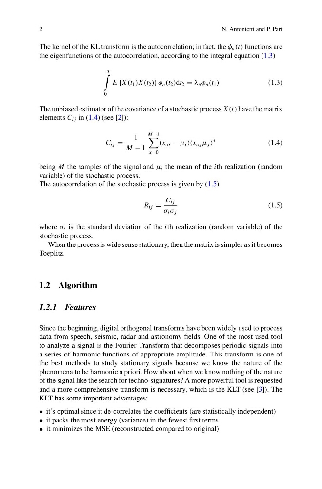
The kernel of the KL transform is the autocorrelation; in fact, the φ n (t) functions are
the eigenfunctions of the autocorrelation, according to the integral equation (1.3)
T
0
E {X (t 1 )X (t 2 )} φ n (t 2 )dt 2 = λ n φ n (t 1 )
(1.3)
The unbiased estimator of the covariance of a stochastic process X (t) have the matrix
elements C i j in (1.4) (see [2]):
C i j =
1
M − 1
M−1
α=0
(x αi − μ i )(x α j μ j )
∗
(1.4)
being M the samples of the signal and μ i the mean of the ith realization (random
variable) of the stochastic process.
The autocorrelation of the stochastic process is given by (1.5)
R i j =
C i j
σ i σ j
(1.5)
where σ i is the standard deviation of the ith realization (random variable) of the
stochastic process.
When the process is wide sense stationary, then the matrix is simpler as it becomes
Toeplitz.
1.2 Algorithm
1.2.1 Features
Since the beginning, digital orthogonal transforms have been widely used to process
data from speech, seismic, radar and astronomy fields. One of the most used tool
to analyze a signal is the Fourier Transform that decomposes periodic signals into
a series of harmonic functions of appropriate amplitude. This transform is one of
the best methods to study stationary signals because we know the nature of the
phenomena to be harmonic a priori. How about when we know nothing of the nature
of the signal like the search for techno-signatures? A more powerful tool is requested
and a more comprehensive transform is necessary, which is the KLT (see [3]). The
KLT has some important advantages:
• it’s optimal since it de-correlates the coefficients (are statistically independent)
• it packs the most energy (variance) in the fewest first terms
• it minimizes the MSE (reconstructed compared to original)
N. Antonietti and P. Pari
The kernel of the KL transform is the autocorrelation; in fact, the φ n (t) functions are
the eigenfunctions of the autocorrelation, according to the integral equation (1.3)
T
0
E {X (t 1 )X (t 2 )} φ n (t 2 )dt 2 = λ n φ n (t 1 )
(1.3)
The unbiased estimator of the covariance of a stochastic process X (t) have the matrix
elements C i j in (1.4) (see [2]):
C i j =
1
M − 1
M−1
α=0
(x αi − μ i )(x α j μ j )
∗
(1.4)
being M the samples of the signal and μ i the mean of the ith realization (random
variable) of the stochastic process.
The autocorrelation of the stochastic process is given by (1.5)
R i j =
C i j
σ i σ j
(1.5)
where σ i is the standard deviation of the ith realization (random variable) of the
stochastic process.
When the process is wide sense stationary, then the matrix is simpler as it becomes
Toeplitz.
1.2 Algorithm
1.2.1 Features
Since the beginning, digital orthogonal transforms have been widely used to process
data from speech, seismic, radar and astronomy fields. One of the most used tool
to analyze a signal is the Fourier Transform that decomposes periodic signals into
a series of harmonic functions of appropriate amplitude. This transform is one of
the best methods to study stationary signals because we know the nature of the
phenomena to be harmonic a priori. How about when we know nothing of the nature
of the signal like the search for techno-signatures? A more powerful tool is requested
and a more comprehensive transform is necessary, which is the KLT (see [3]). The
KLT has some important advantages:
• it’s optimal since it de-correlates the coefficients (are statistically independent)
• it packs the most energy (variance) in the fewest first terms
• it minimizes the MSE (reconstructed compared to original)