

3 Reduced Phase Models of Oscillatory Neural Networks
43
-0.2
0
0.2
0.4
0.6
0.8
1
0
0.1
0.2
0.3
0.4
0.5
0.6
0.7
0.8
0.9
1
E
1,2
(a)
Bifurcation diagram
(b) Dynamics in E-I space
(c) Mean phase dynamics
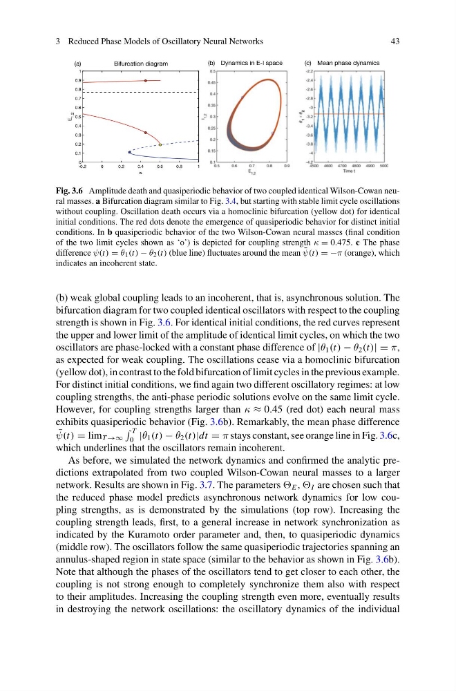
Fig. 3.6 Amplitude death and quasiperiodic behavior of two coupled identical Wilson-Cowan neural masses. a Bifurcation diagram similar to Fig. 3.4, but starting with stable limit cycle oscillations
without coupling. Oscillation death occurs via a homoclinic bifurcation (yellow dot) for identical
initial conditions. The red dots denote the emergence of quasiperiodic behavior for distinct initial
conditions. In b quasiperiodic behavior of the two Wilson-Cowan neural masses (final condition
of the two limit cycles shown as ‘o’) is depicted for coupling strength κ = 0.475. c The phase
difference ψ(t) = θ 1 (t) − θ 2 (t) (blue line) fluctuates around the mean ¯
ψ(t) = −π (orange), which
indicates an incoherent state.
(b) weak global coupling leads to an incoherent, that is, asynchronous solution. The
bifurcation diagram for two coupled identical oscillators with respect to the coupling
strength is shown in Fig. 3.6. For identical initial conditions, the red curves represent
the upper and lower limit of the amplitude of identical limit cycles, on which the two
oscillators are phase-locked with a constant phase difference of |θ 1 (t) − θ 2 (t)| = π,
as expected for weak coupling. The oscillations cease via a homoclinic bifurcation
(yellow dot), in contrast to the fold bifurcation of limit cycles in the previous example.
For distinct initial conditions, we find again two different oscillatory regimes: at low
coupling strengths, the anti-phase periodic solutions evolve on the same limit cycle.
However, for coupling strengths larger than κ ≈ 0.45 (red dot) each neural mass
exhibits quasiperiodic behavior (Fig. 3.6b). Remarkably, the mean phase difference
¯
ψ(t) = lim T →∞
T
0 |θ 1 (t) − θ 2 (t)|dt = π stays constant, see orange line in Fig. 3.6c,
which underlines that the oscillators remain incoherent.
As before, we simulated the network dynamics and confirmed the analytic predictions extrapolated from two coupled Wilson-Cowan neural masses to a larger
network. Results are shown in Fig. 3.7. The parameters E , , I are chosen such that
the reduced phase model predicts asynchronous network dynamics for low coupling strengths, as is demonstrated by the simulations (top row). Increasing the
coupling strength leads, first, to a general increase in network synchronization as
indicated by the Kuramoto order parameter and, then, to quasiperiodic dynamics
(middle row). The oscillators follow the same quasiperiodic trajectories spanning an
annulus-shaped region in state space (similar to the behavior as shown in Fig. 3.6b).
Note that although the phases of the oscillators tend to get closer to each other, the
coupling is not strong enough to completely synchronize them also with respect
to their amplitudes. Increasing the coupling strength even more, eventually results
in destroying the network oscillations: the oscillatory dynamics of the individual
43
-0.2
0
0.2
0.4
0.6
0.8
1
0
0.1
0.2
0.3
0.4
0.5
0.6
0.7
0.8
0.9
1
E
1,2
(a)
Bifurcation diagram
(b) Dynamics in E-I space
(c) Mean phase dynamics
Fig. 3.6 Amplitude death and quasiperiodic behavior of two coupled identical Wilson-Cowan neural masses. a Bifurcation diagram similar to Fig. 3.4, but starting with stable limit cycle oscillations
without coupling. Oscillation death occurs via a homoclinic bifurcation (yellow dot) for identical
initial conditions. The red dots denote the emergence of quasiperiodic behavior for distinct initial
conditions. In b quasiperiodic behavior of the two Wilson-Cowan neural masses (final condition
of the two limit cycles shown as ‘o’) is depicted for coupling strength κ = 0.475. c The phase
difference ψ(t) = θ 1 (t) − θ 2 (t) (blue line) fluctuates around the mean ¯
ψ(t) = −π (orange), which
indicates an incoherent state.
(b) weak global coupling leads to an incoherent, that is, asynchronous solution. The
bifurcation diagram for two coupled identical oscillators with respect to the coupling
strength is shown in Fig. 3.6. For identical initial conditions, the red curves represent
the upper and lower limit of the amplitude of identical limit cycles, on which the two
oscillators are phase-locked with a constant phase difference of |θ 1 (t) − θ 2 (t)| = π,
as expected for weak coupling. The oscillations cease via a homoclinic bifurcation
(yellow dot), in contrast to the fold bifurcation of limit cycles in the previous example.
For distinct initial conditions, we find again two different oscillatory regimes: at low
coupling strengths, the anti-phase periodic solutions evolve on the same limit cycle.
However, for coupling strengths larger than κ ≈ 0.45 (red dot) each neural mass
exhibits quasiperiodic behavior (Fig. 3.6b). Remarkably, the mean phase difference
¯
ψ(t) = lim T →∞
T
0 |θ 1 (t) − θ 2 (t)|dt = π stays constant, see orange line in Fig. 3.6c,
which underlines that the oscillators remain incoherent.
As before, we simulated the network dynamics and confirmed the analytic predictions extrapolated from two coupled Wilson-Cowan neural masses to a larger
network. Results are shown in Fig. 3.7. The parameters E , , I are chosen such that
the reduced phase model predicts asynchronous network dynamics for low coupling strengths, as is demonstrated by the simulations (top row). Increasing the
coupling strength leads, first, to a general increase in network synchronization as
indicated by the Kuramoto order parameter and, then, to quasiperiodic dynamics
(middle row). The oscillators follow the same quasiperiodic trajectories spanning an
annulus-shaped region in state space (similar to the behavior as shown in Fig. 3.6b).
Note that although the phases of the oscillators tend to get closer to each other, the
coupling is not strong enough to completely synchronize them also with respect
to their amplitudes. Increasing the coupling strength even more, eventually results
in destroying the network oscillations: the oscillatory dynamics of the individual