

3 Reduced Phase Models of Oscillatory Neural Networks
37
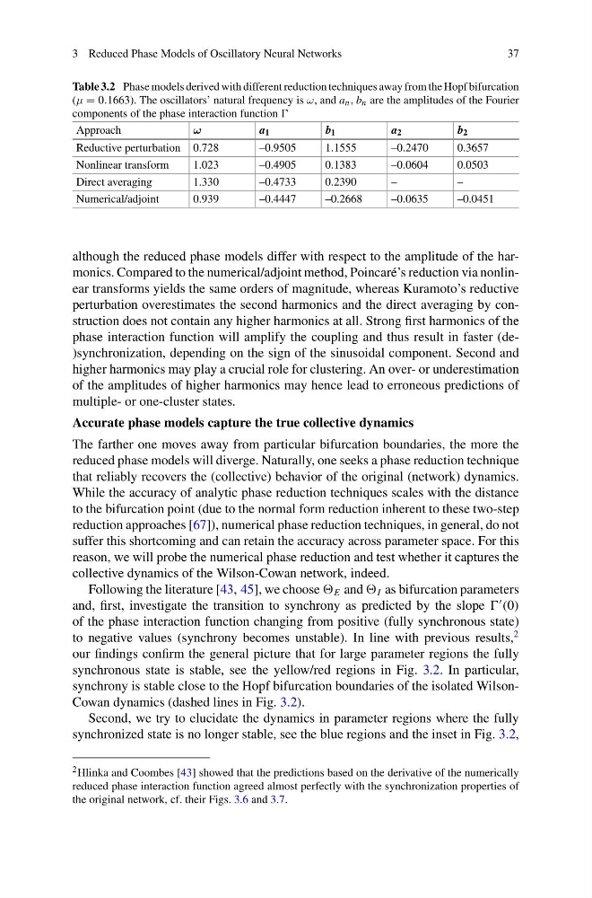
Table 3.2 Phase models derived with different reduction techniques away from the Hopf bifurcation
(μ = 0.1663). The oscillators’ natural frequency is ω, and a n , b n are the amplitudes of the Fourier
components of the phase interaction function
Approach
ω
a 1
b 1
a 2
b 2
Reductive perturbation 0.728
–0.9505
1.1555
–0.2470
0.3657
Nonlinear transform
1.023
–0.4905
0.1383
–0.0604
0.0503
Direct averaging
1.330
–0.4733
0.2390
–
–
Numerical/adjoint
0.939
–0.4447
–0.2668
–0.0635
–0.0451
although the reduced phase models differ with respect to the amplitude of the harmonics. Compared to the numerical/adjoint method, Poincaré’s reduction via nonlinear transforms yields the same orders of magnitude, whereas Kuramoto’s reductive
perturbation overestimates the second harmonics and the direct averaging by construction does not contain any higher harmonics at all. Strong first harmonics of the
phase interaction function will amplify the coupling and thus result in faster (de)synchronization, depending on the sign of the sinusoidal component. Second and
higher harmonics may play a crucial role for clustering. An over- or underestimation
of the amplitudes of higher harmonics may hence lead to erroneous predictions of
multiple- or one-cluster states.
Accurate phase models capture the true collective dynamics
The farther one moves away from particular bifurcation boundaries, the more the
reduced phase models will diverge. Naturally, one seeks a phase reduction technique
that reliably recovers the (collective) behavior of the original (network) dynamics.
While the accuracy of analytic phase reduction techniques scales with the distance
to the bifurcation point (due to the normal form reduction inherent to these two-step
reduction approaches [67]), numerical phase reduction techniques, in general, do not
suffer this shortcoming and can retain the accuracy across parameter space. For this
reason, we will probe the numerical phase reduction and test whether it captures the
collective dynamics of the Wilson-Cowan network, indeed.
Following the literature [43, 45], we choose E and I as bifurcation parameters
and, first, investigate the transition to synchrony as predicted by the slope
(0)
of the phase interaction function changing from positive (fully synchronous state)
to negative values (synchrony becomes unstable). In line with previous results,
2
our findings confirm the general picture that for large parameter regions the fully
synchronous state is stable, see the yellow/red regions in Fig. 3.2. In particular,
synchrony is stable close to the Hopf bifurcation boundaries of the isolated WilsonCowan dynamics (dashed lines in Fig. 3.2).
Second, we try to elucidate the dynamics in parameter regions where the fully
synchronized state is no longer stable, see the blue regions and the inset in Fig. 3.2,
2 Hlinka and Coombes [43] showed that the predictions based on the derivative of the numerically
reduced phase interaction function agreed almost perfectly with the synchronization properties of
the original network, cf. their Figs. 3.6 and 3.7.
37
Table 3.2 Phase models derived with different reduction techniques away from the Hopf bifurcation
(μ = 0.1663). The oscillators’ natural frequency is ω, and a n , b n are the amplitudes of the Fourier
components of the phase interaction function
Approach
ω
a 1
b 1
a 2
b 2
Reductive perturbation 0.728
–0.9505
1.1555
–0.2470
0.3657
Nonlinear transform
1.023
–0.4905
0.1383
–0.0604
0.0503
Direct averaging
1.330
–0.4733
0.2390
–
–
Numerical/adjoint
0.939
–0.4447
–0.2668
–0.0635
–0.0451
although the reduced phase models differ with respect to the amplitude of the harmonics. Compared to the numerical/adjoint method, Poincaré’s reduction via nonlinear transforms yields the same orders of magnitude, whereas Kuramoto’s reductive
perturbation overestimates the second harmonics and the direct averaging by construction does not contain any higher harmonics at all. Strong first harmonics of the
phase interaction function will amplify the coupling and thus result in faster (de)synchronization, depending on the sign of the sinusoidal component. Second and
higher harmonics may play a crucial role for clustering. An over- or underestimation
of the amplitudes of higher harmonics may hence lead to erroneous predictions of
multiple- or one-cluster states.
Accurate phase models capture the true collective dynamics
The farther one moves away from particular bifurcation boundaries, the more the
reduced phase models will diverge. Naturally, one seeks a phase reduction technique
that reliably recovers the (collective) behavior of the original (network) dynamics.
While the accuracy of analytic phase reduction techniques scales with the distance
to the bifurcation point (due to the normal form reduction inherent to these two-step
reduction approaches [67]), numerical phase reduction techniques, in general, do not
suffer this shortcoming and can retain the accuracy across parameter space. For this
reason, we will probe the numerical phase reduction and test whether it captures the
collective dynamics of the Wilson-Cowan network, indeed.
Following the literature [43, 45], we choose E and I as bifurcation parameters
and, first, investigate the transition to synchrony as predicted by the slope
(0)
of the phase interaction function changing from positive (fully synchronous state)
to negative values (synchrony becomes unstable). In line with previous results,
2
our findings confirm the general picture that for large parameter regions the fully
synchronous state is stable, see the yellow/red regions in Fig. 3.2. In particular,
synchrony is stable close to the Hopf bifurcation boundaries of the isolated WilsonCowan dynamics (dashed lines in Fig. 3.2).
Second, we try to elucidate the dynamics in parameter regions where the fully
synchronized state is no longer stable, see the blue regions and the inset in Fig. 3.2,
2 Hlinka and Coombes [43] showed that the predictions based on the derivative of the numerically
reduced phase interaction function agreed almost perfectly with the synchronization properties of
the original network, cf. their Figs. 3.6 and 3.7.