

36
B. Pietras and A. Daffertshofer
apply the four different phase reduction techniques to the network of Wilson-Cowan
neural masses Eq. (3.1). In the resulting phase models Eq. (3.2), we will concentrate
on the reduced natural frequency term ω k and the first two Fourier harmonics in the
phase interaction function Eq. (3.3). Their amplitudes will serve as a quantitative
measure of how accurate the phase models are, whereas their relationships with one
another provide a qualitative measure indicating whether the reduced phase models
result in the correctly predicted collective dynamics; see the end of Sect. 3.2 for a
classification of the network’s phase dynamics in terms of the Fourier coefficients.
Phase reduction is highly parameter-sensitive
A first litmus test concerns the accuracy of the different phase reduction techniques
close to a bifurcation boundary. Center manifold and normal form theory prescribe
the exact form of the phase interaction function (ψ), see [16]. For the regime near
a supercritical Hopf bifurcation, the topological normal form [53] of the dynamics
yields a purely sinusoidal phase interaction function, that is, all Fourier coefficients
but b 1 in Eq. (3.3) will vanish. The topological Hopf normal form requires further
algebraic transformations than the conventional (Poincaré) Hopf normal form, but
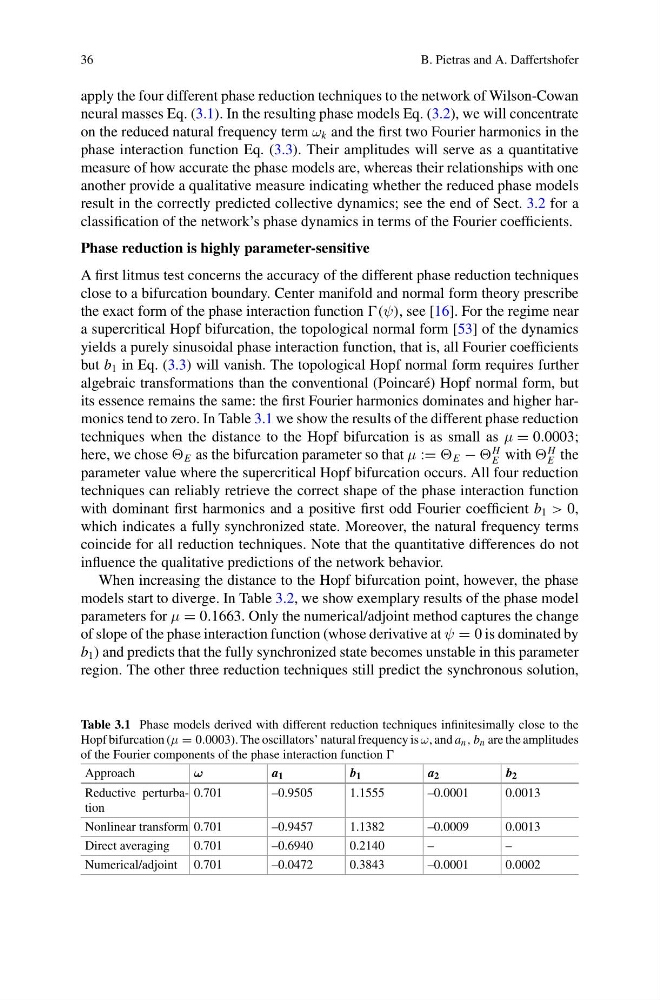
its essence remains the same: the first Fourier harmonics dominates and higher harmonics tend to zero. In Table 3.1 we show the results of the different phase reduction
techniques when the distance to the Hopf bifurcation is as small as μ = 0.0003;
here, we chose E as the bifurcation parameter so that μ := E −
H
E with
H
E the
parameter value where the supercritical Hopf bifurcation occurs. All four reduction
techniques can reliably retrieve the correct shape of the phase interaction function
with dominant first harmonics and a positive first odd Fourier coefficient b 1 > 0,
which indicates a fully synchronized state. Moreover, the natural frequency terms
coincide for all reduction techniques. Note that the quantitative differences do not
influence the qualitative predictions of the network behavior.
When increasing the distance to the Hopf bifurcation point, however, the phase
models start to diverge. In Table 3.2, we show exemplary results of the phase model
parameters for μ = 0.1663. Only the numerical/adjoint method captures the change
of slope of the phase interaction function (whose derivative at ψ = 0 is dominated by
b 1 ) and predicts that the fully synchronized state becomes unstable in this parameter
region. The other three reduction techniques still predict the synchronous solution,
Table 3.1 Phase models derived with different reduction techniques infinitesimally close to the
Hopf bifurcation (μ = 0.0003). The oscillators’ natural frequency is ω, and a n , b n are the amplitudes
of the Fourier components of the phase interaction function
Approach
ω
a 1
b 1
a 2
b 2
Reductive perturbation
0.701
–0.9505
1.1555
–0.0001
0.0013
Nonlinear transform 0.701
–0.9457
1.1382
–0.0009
0.0013
Direct averaging
0.701
–0.6940
0.2140
–
–
Numerical/adjoint 0.701
–0.0472
0.3843
–0.0001
0.0002
B. Pietras and A. Daffertshofer
apply the four different phase reduction techniques to the network of Wilson-Cowan
neural masses Eq. (3.1). In the resulting phase models Eq. (3.2), we will concentrate
on the reduced natural frequency term ω k and the first two Fourier harmonics in the
phase interaction function Eq. (3.3). Their amplitudes will serve as a quantitative
measure of how accurate the phase models are, whereas their relationships with one
another provide a qualitative measure indicating whether the reduced phase models
result in the correctly predicted collective dynamics; see the end of Sect. 3.2 for a
classification of the network’s phase dynamics in terms of the Fourier coefficients.
Phase reduction is highly parameter-sensitive
A first litmus test concerns the accuracy of the different phase reduction techniques
close to a bifurcation boundary. Center manifold and normal form theory prescribe
the exact form of the phase interaction function (ψ), see [16]. For the regime near
a supercritical Hopf bifurcation, the topological normal form [53] of the dynamics
yields a purely sinusoidal phase interaction function, that is, all Fourier coefficients
but b 1 in Eq. (3.3) will vanish. The topological Hopf normal form requires further
algebraic transformations than the conventional (Poincaré) Hopf normal form, but
its essence remains the same: the first Fourier harmonics dominates and higher harmonics tend to zero. In Table 3.1 we show the results of the different phase reduction
techniques when the distance to the Hopf bifurcation is as small as μ = 0.0003;
here, we chose E as the bifurcation parameter so that μ := E −
H
E with
H
E the
parameter value where the supercritical Hopf bifurcation occurs. All four reduction
techniques can reliably retrieve the correct shape of the phase interaction function
with dominant first harmonics and a positive first odd Fourier coefficient b 1 > 0,
which indicates a fully synchronized state. Moreover, the natural frequency terms
coincide for all reduction techniques. Note that the quantitative differences do not
influence the qualitative predictions of the network behavior.
When increasing the distance to the Hopf bifurcation point, however, the phase
models start to diverge. In Table 3.2, we show exemplary results of the phase model
parameters for μ = 0.1663. Only the numerical/adjoint method captures the change
of slope of the phase interaction function (whose derivative at ψ = 0 is dominated by
b 1 ) and predicts that the fully synchronized state becomes unstable in this parameter
region. The other three reduction techniques still predict the synchronous solution,
Table 3.1 Phase models derived with different reduction techniques infinitesimally close to the
Hopf bifurcation (μ = 0.0003). The oscillators’ natural frequency is ω, and a n , b n are the amplitudes
of the Fourier components of the phase interaction function
Approach
ω
a 1
b 1
a 2
b 2
Reductive perturbation
0.701
–0.9505
1.1555
–0.0001
0.0013
Nonlinear transform 0.701
–0.9457
1.1382
–0.0009
0.0013
Direct averaging
0.701
–0.6940
0.2140
–
–
Numerical/adjoint 0.701
–0.0472
0.3843
–0.0001
0.0002