

3 Reduced Phase Models of Oscillatory Neural Networks
35
˙
x k = Lx k + T
−1 f (T x k ; μ) + κ T
−1
N
j=1
g
T x k , T x j
.
(3.6)
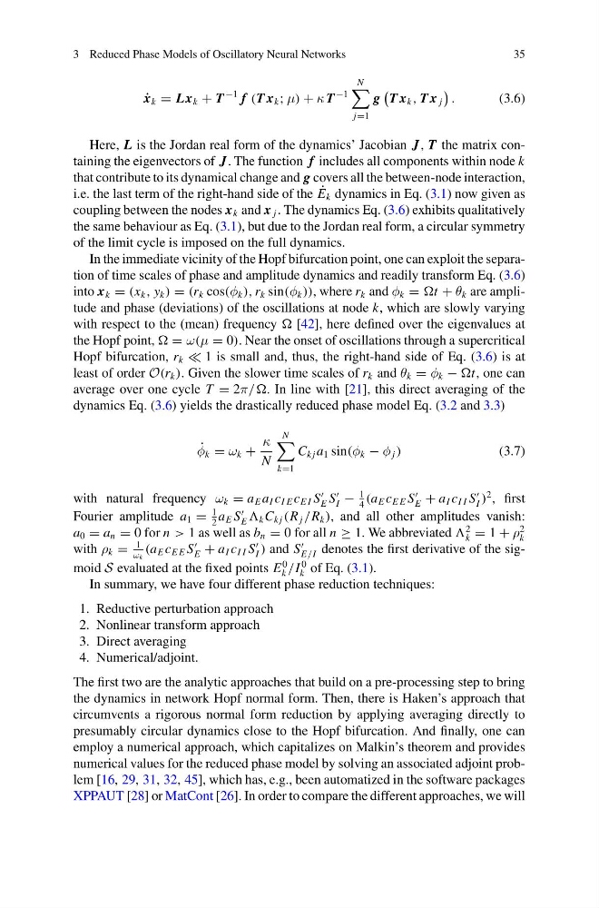
Here, L is the Jordan real form of the dynamics’ Jacobian J, T the matrix containing the eigenvectors of J. The function f includes all components within node k
that contribute to its dynamical change and g covers all the between-node interaction,
i.e. the last term of the right-hand side of the ˙
E k dynamics in Eq. (3.1) now given as
coupling between the nodes x k and x j . The dynamics Eq. (3.6) exhibits qualitatively
the same behaviour as Eq. (3.1), but due to the Jordan real form, a circular symmetry
of the limit cycle is imposed on the full dynamics.
In the immediate vicinity of the Hopf bifurcation point, one can exploit the separation of time scales of phase and amplitude dynamics and readily transform Eq. (3.6)
into x k = (x k , y k ) = (r k cos(φ k ), r k sin(φ k )), where r k and φ k = t + θ k are amplitude and phase (deviations) of the oscillations at node k, which are slowly varying
with respect to the (mean) frequency [42], here defined over the eigenvalues at
the Hopf point, = ω(μ = 0). Near the onset of oscillations through a supercritical
Hopf bifurcation, r k 1 is small and, thus, the right-hand side of Eq. (3.6) is at
least of order O(r k ). Given the slower time scales of r k and θ k = φ k − t, one can
average over one cycle T = 2π//. In line with [21], this direct averaging of the
dynamics Eq. (3.6) yields the drastically reduced phase model Eq. (3.2 and 3.3)
˙
φ k = ω k +
κ
N
N
k=1
C k j a 1 sin(φ k − φ j )
(3.7)
with natural frequency ω k = a E a I c I E c E I S
E S
I −
1
4
(a E c E E S
E + a I c I I S
I )
2 , first
Fourier amplitude a 1 =
1
2
a E S
E k C k j (R j /R k ), and all other amplitudes vanish:
a 0 = a n = 0 for n > 1 as well as b n = 0 for all n ≥ 1. We abbreviated
2
k = 1 + ρ
2
k
with ρ k =
1
ω k
(a E c E E S
E + a I c I I S
I ) and S
E/I denotes the first derivative of the sigmoid S evaluated at the fixed points E
0
k /I
0
k of Eq. (3.1).
In summary, we have four different phase reduction techniques:
1. Reductive perturbation approach
2. Nonlinear transform approach
3. Direct averaging
4. Numerical/adjoint.
The first two are the analytic approaches that build on a pre-processing step to bring
the dynamics in network Hopf normal form. Then, there is Haken’s approach that
circumvents a rigorous normal form reduction by applying averaging directly to
presumably circular dynamics close to the Hopf bifurcation. And finally, one can
employ a numerical approach, which capitalizes on Malkin’s theorem and provides
numerical values for the reduced phase model by solving an associated adjoint problem [16, 29, 31, 32, 45], which has, e.g., been automatized in the software packages
XPPAUT [28] or MatCont [26]. In order to compare the different approaches, we will
35
˙
x k = Lx k + T
−1 f (T x k ; μ) + κ T
−1
N
j=1
g
T x k , T x j
.
(3.6)
Here, L is the Jordan real form of the dynamics’ Jacobian J, T the matrix containing the eigenvectors of J. The function f includes all components within node k
that contribute to its dynamical change and g covers all the between-node interaction,
i.e. the last term of the right-hand side of the ˙
E k dynamics in Eq. (3.1) now given as
coupling between the nodes x k and x j . The dynamics Eq. (3.6) exhibits qualitatively
the same behaviour as Eq. (3.1), but due to the Jordan real form, a circular symmetry
of the limit cycle is imposed on the full dynamics.
In the immediate vicinity of the Hopf bifurcation point, one can exploit the separation of time scales of phase and amplitude dynamics and readily transform Eq. (3.6)
into x k = (x k , y k ) = (r k cos(φ k ), r k sin(φ k )), where r k and φ k = t + θ k are amplitude and phase (deviations) of the oscillations at node k, which are slowly varying
with respect to the (mean) frequency [42], here defined over the eigenvalues at
the Hopf point, = ω(μ = 0). Near the onset of oscillations through a supercritical
Hopf bifurcation, r k 1 is small and, thus, the right-hand side of Eq. (3.6) is at
least of order O(r k ). Given the slower time scales of r k and θ k = φ k − t, one can
average over one cycle T = 2π//. In line with [21], this direct averaging of the
dynamics Eq. (3.6) yields the drastically reduced phase model Eq. (3.2 and 3.3)
˙
φ k = ω k +
κ
N
N
k=1
C k j a 1 sin(φ k − φ j )
(3.7)
with natural frequency ω k = a E a I c I E c E I S
E S
I −
1
4
(a E c E E S
E + a I c I I S
I )
2 , first
Fourier amplitude a 1 =
1
2
a E S
E k C k j (R j /R k ), and all other amplitudes vanish:
a 0 = a n = 0 for n > 1 as well as b n = 0 for all n ≥ 1. We abbreviated
2
k = 1 + ρ
2
k
with ρ k =
1
ω k
(a E c E E S
E + a I c I I S
I ) and S
E/I denotes the first derivative of the sigmoid S evaluated at the fixed points E
0
k /I
0
k of Eq. (3.1).
In summary, we have four different phase reduction techniques:
1. Reductive perturbation approach
2. Nonlinear transform approach
3. Direct averaging
4. Numerical/adjoint.
The first two are the analytic approaches that build on a pre-processing step to bring
the dynamics in network Hopf normal form. Then, there is Haken’s approach that
circumvents a rigorous normal form reduction by applying averaging directly to
presumably circular dynamics close to the Hopf bifurcation. And finally, one can
employ a numerical approach, which capitalizes on Malkin’s theorem and provides
numerical values for the reduced phase model by solving an associated adjoint problem [16, 29, 31, 32, 45], which has, e.g., been automatized in the software packages
XPPAUT [28] or MatCont [26]. In order to compare the different approaches, we will