

2 Phase and Amplitude Description of Complex Oscillatory Patterns …
23
(a)
(b)
0
500
1000
t / T
-
0
0
500
1000
t / T
-
0
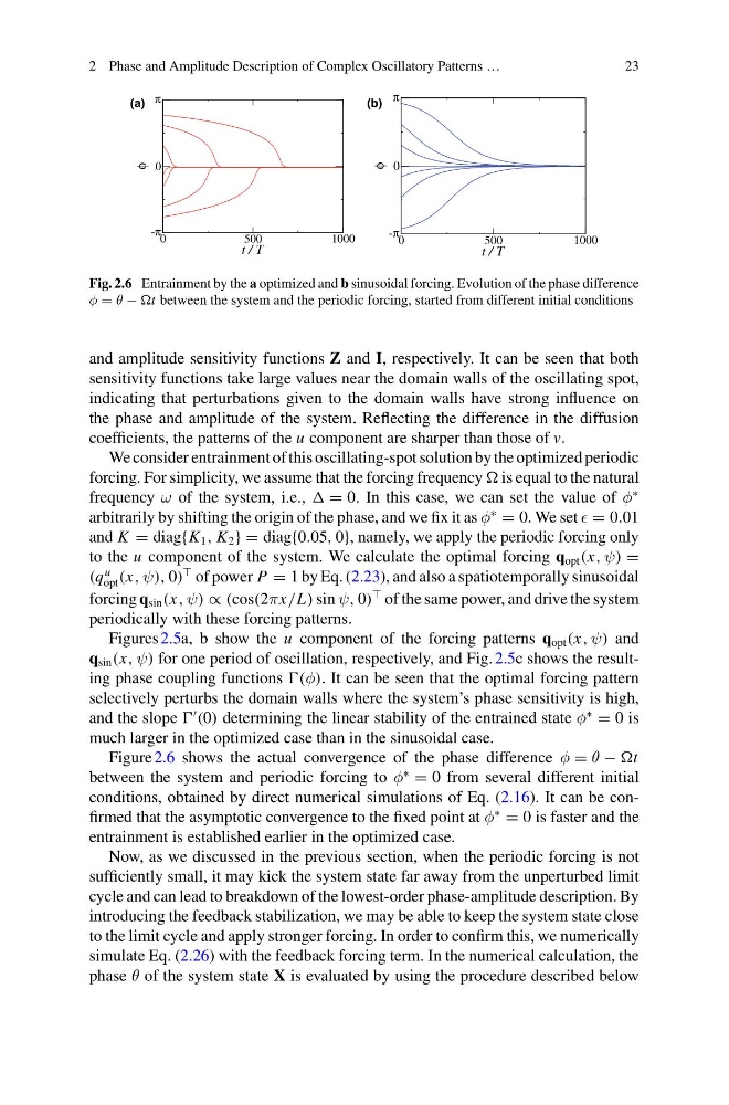
Fig. 2.6 Entrainment by the a optimized and b sinusoidal forcing. Evolution of the phase difference
φ = θ − between the system and the periodic forcing, started from different initial conditions
and amplitude sensitivity functions Z and I, respectively. It can be seen that both
sensitivity functions take large values near the domain walls of the oscillating spot,
indicating that perturbations given to the domain walls have strong influence on
the phase and amplitude of the system. Reflecting the difference in the diffusion
coefficients, the patterns of the u component are sharper than those of v.
We consider entrainment of this oscillating-spot solution by the optimized periodic
forcing. For simplicity, we assume that the forcing frequency is equal to the natural
frequency ω of the system, i.e., = 0. In this case, we can set the value of φ
∗
arbitrarily by shifting the origin of the phase, and we fix it as φ
∗
= 0. We set = 0.01
and K = diag{K 1 , K 2 } = diag{0.05, 0}, namely, we apply the periodic forcing only
to the u component of the system. We calculate the optimal forcing q opt (x, ψ) =
(q
u
opt (x, ψ), 0)
of power P = 1 by Eq. (2.23), and also a spatiotemporally sinusoidal
forcing q sin (x, ψ) ∝ (cos(2πx/L) sin ψ, 0)
of the same power, and drive the system
periodically with these forcing patterns.
Figures 2.5a, b show the u component of the forcing patterns q opt (x, ψ) and
q sin (x, ψ) for one period of oscillation, respectively, and Fig. 2.5c shows the resulting phase coupling functions It can be seen that the optimal forcing pattern
selectively perturbs the domain walls where the system’s phase sensitivity is high,
and the slope
(0) determining the linear stability of the entrained state φ
∗
= 0 is
much larger in the optimized case than in the sinusoidal case.
Figure 2.6 shows the actual convergence of the phase difference φ = θ −
between the system and periodic forcing to φ
∗
= 0 from several different initial
conditions, obtained by direct numerical simulations of Eq. (2.16). It can be confirmed that the asymptotic convergence to the fixed point at φ
∗
= 0 is faster and the
entrainment is established earlier in the optimized case.
Now, as we discussed in the previous section, when the periodic forcing is not
sufficiently small, it may kick the system state far away from the unperturbed limit
cycle and can lead to breakdown of the lowest-order phase-amplitude description. By
introducing the feedback stabilization, we may be able to keep the system state close
to the limit cycle and apply stronger forcing. In order to confirm this, we numerically
simulate Eq. (2.26) with the feedback forcing term. In the numerical calculation, the
phase θ of the system state X is evaluated by using the procedure described below
23
(a)
(b)
0
500
1000
t / T
-
0
0
500
1000
t / T
-
0
Fig. 2.6 Entrainment by the a optimized and b sinusoidal forcing. Evolution of the phase difference
φ = θ − between the system and the periodic forcing, started from different initial conditions
and amplitude sensitivity functions Z and I, respectively. It can be seen that both
sensitivity functions take large values near the domain walls of the oscillating spot,
indicating that perturbations given to the domain walls have strong influence on
the phase and amplitude of the system. Reflecting the difference in the diffusion
coefficients, the patterns of the u component are sharper than those of v.
We consider entrainment of this oscillating-spot solution by the optimized periodic
forcing. For simplicity, we assume that the forcing frequency is equal to the natural
frequency ω of the system, i.e., = 0. In this case, we can set the value of φ
∗
arbitrarily by shifting the origin of the phase, and we fix it as φ
∗
= 0. We set = 0.01
and K = diag{K 1 , K 2 } = diag{0.05, 0}, namely, we apply the periodic forcing only
to the u component of the system. We calculate the optimal forcing q opt (x, ψ) =
(q
u
opt (x, ψ), 0)
of power P = 1 by Eq. (2.23), and also a spatiotemporally sinusoidal
forcing q sin (x, ψ) ∝ (cos(2πx/L) sin ψ, 0)
of the same power, and drive the system
periodically with these forcing patterns.
Figures 2.5a, b show the u component of the forcing patterns q opt (x, ψ) and
q sin (x, ψ) for one period of oscillation, respectively, and Fig. 2.5c shows the resulting phase coupling functions It can be seen that the optimal forcing pattern
selectively perturbs the domain walls where the system’s phase sensitivity is high,
and the slope
(0) determining the linear stability of the entrained state φ
∗
= 0 is
much larger in the optimized case than in the sinusoidal case.
Figure 2.6 shows the actual convergence of the phase difference φ = θ −
between the system and periodic forcing to φ
∗
= 0 from several different initial
conditions, obtained by direct numerical simulations of Eq. (2.16). It can be confirmed that the asymptotic convergence to the fixed point at φ
∗
= 0 is faster and the
entrainment is established earlier in the optimized case.
Now, as we discussed in the previous section, when the periodic forcing is not
sufficiently small, it may kick the system state far away from the unperturbed limit
cycle and can lead to breakdown of the lowest-order phase-amplitude description. By
introducing the feedback stabilization, we may be able to keep the system state close
to the limit cycle and apply stronger forcing. In order to confirm this, we numerically
simulate Eq. (2.26) with the feedback forcing term. In the numerical calculation, the
phase θ of the system state X is evaluated by using the procedure described below