

24
H. Nakao
(a)
(b)
-1
-0.5
0
0.5
1
u(L/3)
-0.4
-0.3
-0.2
-0.1
0
0.1
v(L/3)
K 1 =0.5, =0
K 1 =0.5, =10
unperturbed
0
500
1000
t / T
0
/2
K 1 =0.05, =0
K 1 =0.5, =0
K 1 =0.5, =10
= 0
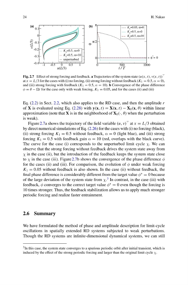
Fig. 2.7 Effect of strong forcing and feedback. a Trajectories of the system state (u(x, t), v(x, t))
at x = L/3 for the cases with (i) no forcing, (ii) strong forcing without feedback (K 1 = 0.5, α = 0),
and (iii) strong forcing with feedback (K 1 = 0.5, α = 10). b Convergence of the phase difference
φ = θ − for the case only with weak forcing, K 1 = 0.05, and for the cases (ii) and (iii)
Eq. (2.2) in Sect. 2.2, which also applies to the RD case, and then the amplitude r
of X is evaluated using Eq. (2.28) with y(x, t) = X(x, t) − X 0 (x, θ) within linear
approximation (note that X is in the neighborhood of X 0 (·, θ) when the perturbation
is weak).
Figure 2.7a shows the trajectory of the field variable (u, v)
at x = L/3 obtained
by direct numerical simulations of Eq. (2.26) for the cases with (i) no forcing (black),
(ii) strong forcing K 1 = 0.5 without feedback, α = 0 (light blue), and (iii) strong
forcing K 1 = 0.5 with feedback gain α = 10 (red, overlaps with the black curve).
The curve for the case (i) corresponds to the unperturbed limit cycle χ. We can
observe that the strong forcing without feedback drives the system state away from
χ in the case (ii), but the introduction of the feedback keeps the system state close
to χ in the case (iii). Figure 2.7b shows the convergence of the phase difference φ
for the cases (ii) and (iii). For comparison, the evolution of φ under weak forcing
K 1 = 0.05 without feedback is also shown. In the case (ii) without feedback, the
final phase difference is considerably different from the target value φ
∗
= 0 because
of the large deviation of the system state from χ.
3 In contrast, in the case (iii) with
feedback, φ converges to the correct target value φ
∗
= 0 even though the forcing is
10 times stronger. Thus, the feedback stabilization allows us to apply much stronger
periodic forcing and realize faster entrainment.
2.6 Summary
We have formulated the method of phase and amplitude description for limit-cycle
oscillations in spatially extended RD systems subjected to weak perturbations.
Though the RD systems are infinite-dimensional dynamical systems, we can still
3 In this case, the system state converges to a spurious periodic orbit after initial transient, which is
induced by the effect of the strong periodic forcing and larger than the original limit cycle χ.
H. Nakao
(a)
(b)
-1
-0.5
0
0.5
1
u(L/3)
-0.4
-0.3
-0.2
-0.1
0
0.1
v(L/3)
K 1 =0.5, =0
K 1 =0.5, =10
unperturbed
0
500
1000
t / T
0
/2
K 1 =0.05, =0
K 1 =0.5, =0
K 1 =0.5, =10
= 0
Fig. 2.7 Effect of strong forcing and feedback. a Trajectories of the system state (u(x, t), v(x, t))
at x = L/3 for the cases with (i) no forcing, (ii) strong forcing without feedback (K 1 = 0.5, α = 0),
and (iii) strong forcing with feedback (K 1 = 0.5, α = 10). b Convergence of the phase difference
φ = θ − for the case only with weak forcing, K 1 = 0.05, and for the cases (ii) and (iii)
Eq. (2.2) in Sect. 2.2, which also applies to the RD case, and then the amplitude r
of X is evaluated using Eq. (2.28) with y(x, t) = X(x, t) − X 0 (x, θ) within linear
approximation (note that X is in the neighborhood of X 0 (·, θ) when the perturbation
is weak).
Figure 2.7a shows the trajectory of the field variable (u, v)
at x = L/3 obtained
by direct numerical simulations of Eq. (2.26) for the cases with (i) no forcing (black),
(ii) strong forcing K 1 = 0.5 without feedback, α = 0 (light blue), and (iii) strong
forcing K 1 = 0.5 with feedback gain α = 10 (red, overlaps with the black curve).
The curve for the case (i) corresponds to the unperturbed limit cycle χ. We can
observe that the strong forcing without feedback drives the system state away from
χ in the case (ii), but the introduction of the feedback keeps the system state close
to χ in the case (iii). Figure 2.7b shows the convergence of the phase difference φ
for the cases (ii) and (iii). For comparison, the evolution of φ under weak forcing
K 1 = 0.05 without feedback is also shown. In the case (ii) without feedback, the
final phase difference is considerably different from the target value φ
∗
= 0 because
of the large deviation of the system state from χ.
3 In contrast, in the case (iii) with
feedback, φ converges to the correct target value φ
∗
= 0 even though the forcing is
10 times stronger. Thus, the feedback stabilization allows us to apply much stronger
periodic forcing and realize faster entrainment.
2.6 Summary
We have formulated the method of phase and amplitude description for limit-cycle
oscillations in spatially extended RD systems subjected to weak perturbations.
Though the RD systems are infinite-dimensional dynamical systems, we can still
3 In this case, the system state converges to a spurious periodic orbit after initial transient, which is
induced by the effect of the strong periodic forcing and larger than the original limit cycle χ.