

12 Phase Reconstruction with Iterated Hilbert Transforms
203
κ = 200 to construct ˙
θ(ϕ, η). We apply a simple iterative method described in [19].
After K iterative steps, the extracted coupling function ˜
Q K ,n (ϕ, η) := ˙
θ n (ϕ, η) − ˜
ω
is factorized into ˜
Z K (ϕ) and ˜
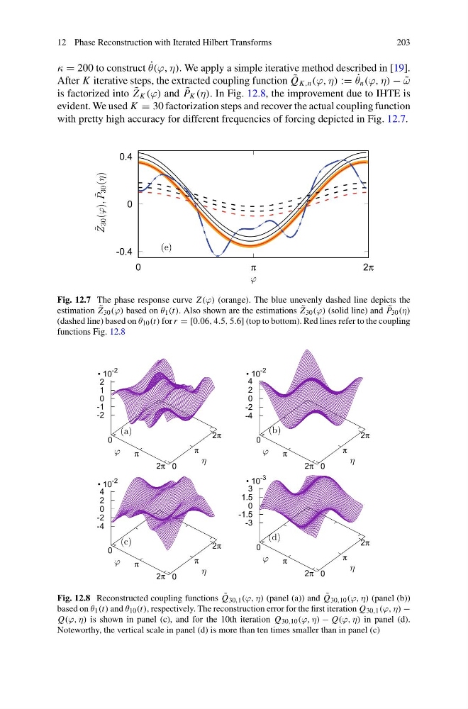
P K (η). In Fig. 12.8, the improvement due to IHTE is
evident. We used K = 30 factorization steps and recover the actual coupling function
with pretty high accuracy for different frequencies of forcing depicted in Fig. 12.7.
-0.4
0
0.4
0
π
2π
˜
Z
30 (ϕ), ˜
P
30 (η)
ϕ
(e)
Fig. 12.7 The phase response curve Z (ϕ) (orange). The blue unevenly dashed line depicts the
estimation ˜
Z 30 (ϕ) based on θ 1 (t). Also shown are the estimations ˜
Z 30 (ϕ) (solid line) and ˜
P 30 (η)
(dashed line) based on θ 10 (t) for r = [0.06, 4.5, 5.6] (top to bottom). Red lines refer to the coupling
functions Fig. 12.8
0
π
2π 0
π
2π
-2
-1
0
1
2
• 10
-2
0
π
2π 0
π
2π
-4
-2
0
2
4
• 10
-2
0
π
2π 0
π
2π
-4
-2
0
2
4
• 10
-2
0
π
2π 0
π
2π
-3
-1.5
0
1.5
3
• 10
-3
(a)
(b)
(c)
(d)
ϕ
ϕ
ϕ
ϕ
η
η
η
η
Fig. 12.8 Reconstructed coupling functions ˜
Q 30,1 (ϕ, η) (panel (a)) and ˜
Q 30,10 (ϕ, η) (panel (b))
based on θ 1 (t) and θ 10 (t), respectively. The reconstruction error for the first iteration Q 30,1 (ϕ, η) −
Q(ϕ, η) is shown in panel (c), and for the 10th iteration Q 30,10 (ϕ, η) − Q(ϕ, η) in panel (d).
Noteworthy, the vertical scale in panel (d) is more than ten times smaller than in panel (c)
203
κ = 200 to construct ˙
θ(ϕ, η). We apply a simple iterative method described in [19].
After K iterative steps, the extracted coupling function ˜
Q K ,n (ϕ, η) := ˙
θ n (ϕ, η) − ˜
ω
is factorized into ˜
Z K (ϕ) and ˜
P K (η). In Fig. 12.8, the improvement due to IHTE is
evident. We used K = 30 factorization steps and recover the actual coupling function
with pretty high accuracy for different frequencies of forcing depicted in Fig. 12.7.
-0.4
0
0.4
0
π
2π
˜
Z
30 (ϕ), ˜
P
30 (η)
ϕ
(e)
Fig. 12.7 The phase response curve Z (ϕ) (orange). The blue unevenly dashed line depicts the
estimation ˜
Z 30 (ϕ) based on θ 1 (t). Also shown are the estimations ˜
Z 30 (ϕ) (solid line) and ˜
P 30 (η)
(dashed line) based on θ 10 (t) for r = [0.06, 4.5, 5.6] (top to bottom). Red lines refer to the coupling
functions Fig. 12.8
0
π
2π 0
π
2π
-2
-1
0
1
2
• 10
-2
0
π
2π 0
π
2π
-4
-2
0
2
4
• 10
-2
0
π
2π 0
π
2π
-4
-2
0
2
4
• 10
-2
0
π
2π 0
π
2π
-3
-1.5
0
1.5
3
• 10
-3
(a)
(b)
(c)
(d)
ϕ
ϕ
ϕ
ϕ
η
η
η
η
Fig. 12.8 Reconstructed coupling functions ˜
Q 30,1 (ϕ, η) (panel (a)) and ˜
Q 30,10 (ϕ, η) (panel (b))
based on θ 1 (t) and θ 10 (t), respectively. The reconstruction error for the first iteration Q 30,1 (ϕ, η) −
Q(ϕ, η) is shown in panel (c), and for the 10th iteration Q 30,10 (ϕ, η) − Q(ϕ, η) in panel (d).
Noteworthy, the vertical scale in panel (d) is more than ten times smaller than in panel (c)