

202
E. Gengel and A. Pikovsky
-0.1
0
0.1
-0.02
0
0.02
1010.0
1050.0
1090.0
0.15
0.20
0.25
0.18
0.20
0.22
1005.0
1025.0
1045.0
time
time
q(t),u
1,10 (t)
q(t),u
1,10 (t)
˙
ϕ(t), ˙
θ
1,10 (t)
˙
ϕ(t), ˙
ψ
1,10 (t)
(a)
(b)
(c)
(d)
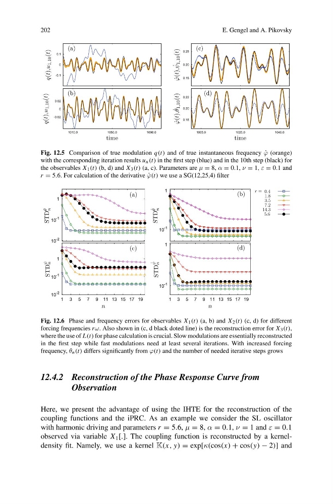
Fig. 12.5 Comparison of true modulation q(t) and of true instantaneous frequency ˙
ϕ (orange)
with the corresponding iteration results u n (t) in the first step (blue) and in the 10th step (black) for
the observables X 1 (t) (b, d) and X 3 (t) (a, c). Parameters are μ = 8, α = 0.1, ν = 1, ε = 0.1 and
r = 5.6. For calculation of the derivative ˙
ϕ(t) we use a SG(12,25,4) filter
10
-2
10
-1
1
10
-1
1
10
-2
10
-1
1
1 3 5 7 9 11 13 15 17 19
10
-1
1
1 3 5 7 9 11 13 15 17 19
n
n
STD θ
n
STD
˙
θ
n
STD
ψ
n
STD
˙
ψ
n
0.4
1.8
3.5
7.2
14.3
5.6
(a)
(b)
(c)
(d)
r =
Fig. 12.6 Phase and frequency errors for observables X 1 (t) (a, b) and X 2 (t) (c, d) for different
forcing frequencies r ω. Also shown in (c, d black doted line) is the reconstruction error for X 3 (t),
where the use of L(t) for phase calculation is crucial. Slow modulations are essentially reconstructed
in the first step while fast modulations need at least several iterations. With increased forcing
frequency, θ n (t) differs significantly from ϕ(t) and the number of needed iterative steps grows
12.4.2 Reconstruction of the Phase Response Curve from
Observation
Here, we present the advantage of using the IHTE for the reconstruction of the
coupling functions and the iPRC. As an example we consider the SL oscillator
with harmonic driving and parameters r = 5.6, μ = 8, α = 0.1, ν = 1 and ε = 0.1
observed via variable X 1 [.]. The coupling function is reconstructed by a kerneldensity fit. Namely, we use a kernel K(x, y) = exp[κ(cos(x) + cos(y) − 2)] and
E. Gengel and A. Pikovsky
-0.1
0
0.1
-0.02
0
0.02
1010.0
1050.0
1090.0
0.15
0.20
0.25
0.18
0.20
0.22
1005.0
1025.0
1045.0
time
time
q(t),u
1,10 (t)
q(t),u
1,10 (t)
˙
ϕ(t), ˙
θ
1,10 (t)
˙
ϕ(t), ˙
ψ
1,10 (t)
(a)
(b)
(c)
(d)
Fig. 12.5 Comparison of true modulation q(t) and of true instantaneous frequency ˙
ϕ (orange)
with the corresponding iteration results u n (t) in the first step (blue) and in the 10th step (black) for
the observables X 1 (t) (b, d) and X 3 (t) (a, c). Parameters are μ = 8, α = 0.1, ν = 1, ε = 0.1 and
r = 5.6. For calculation of the derivative ˙
ϕ(t) we use a SG(12,25,4) filter
10
-2
10
-1
1
10
-1
1
10
-2
10
-1
1
1 3 5 7 9 11 13 15 17 19
10
-1
1
1 3 5 7 9 11 13 15 17 19
n
n
STD θ
n
STD
˙
θ
n
STD
ψ
n
STD
˙
ψ
n
0.4
1.8
3.5
7.2
14.3
5.6
(a)
(b)
(c)
(d)
r =
Fig. 12.6 Phase and frequency errors for observables X 1 (t) (a, b) and X 2 (t) (c, d) for different
forcing frequencies r ω. Also shown in (c, d black doted line) is the reconstruction error for X 3 (t),
where the use of L(t) for phase calculation is crucial. Slow modulations are essentially reconstructed
in the first step while fast modulations need at least several iterations. With increased forcing
frequency, θ n (t) differs significantly from ϕ(t) and the number of needed iterative steps grows
12.4.2 Reconstruction of the Phase Response Curve from
Observation
Here, we present the advantage of using the IHTE for the reconstruction of the
coupling functions and the iPRC. As an example we consider the SL oscillator
with harmonic driving and parameters r = 5.6, μ = 8, α = 0.1, ν = 1 and ε = 0.1
observed via variable X 1 [.]. The coupling function is reconstructed by a kerneldensity fit. Namely, we use a kernel K(x, y) = exp[κ(cos(x) + cos(y) − 2)] and