

204
E. Gengel and A. Pikovsky
12.4.3 Noisy Oscillations
In this section we discuss applicability of the described method to noisy signals. We
assume that the SL oscillator is driven by an external force containing a deterministic
and a stochastic (white noise) component
εP(t) = ε cos(ωrt) + ξ(t),
= 0, ξ(t
) = σ
2
δ(t − t
)
(12.18)
with μ = 8, α = 0.1, ν = 1, ε = 0.2, r = 5.6 and different noise levels σ = [0.1,
0.08, 0.06]. We assume a “perfect” observation according to X 1 (t) (i.e., there is no
observational noise). Due to the stochastic forcing, the signal’s spectrum has infinite
support. In the time domain, X (t) contains an infinite amount of local maxima and
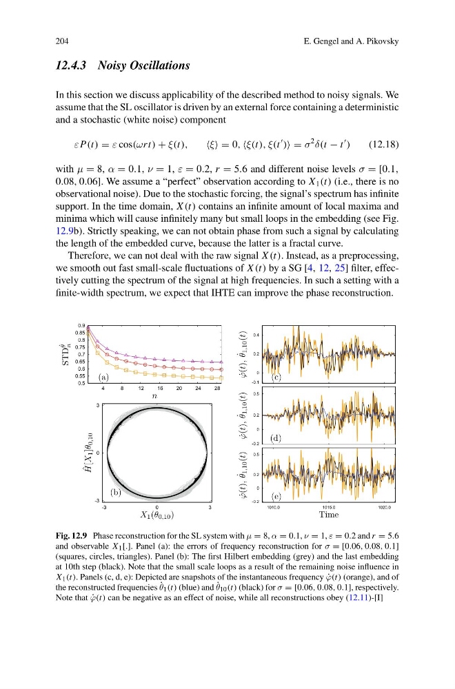
minima which will cause infinitely many but small loops in the embedding (see Fig.
12.9b). Strictly speaking, we can not obtain phase from such a signal by calculating
the length of the embedded curve, because the latter is a fractal curve.
Therefore, we can not deal with the raw signal X (t). Instead, as a preprocessing,
we smooth out fast small-scale fluctuations of X (t) by a SG [4, 12, 25] filter, effectively cutting the spectrum of the signal at high frequencies. In such a setting with a
finite-width spectrum, we expect that IHTE can improve the phase reconstruction.
0.5
0.55
0.6
0.65
0.7
0.75
0.8
0.85
0.9
4
8
12
16
20
24
28
-3
0
3
-3
0
3
-0.1
0
0.2
0.4
-0.2
0
0.2
0.5
-0.2
0
0.2
0.5
1010.0
1015.0
1020.0
Time
˙
ϕ(t), ˙
θ
1,10 (t)
˙
ϕ(t), ˙
θ
1,10 (t)
˙
ϕ(t), ˙
θ
1,10 (t)
n
STD
˙
θ
n
ˆ
H[X
1 ]θ
0,10
X 1 (θ 0,10 )
(a)
(b)
(c)
(d)
(e)
Fig. 12.9 Phase reconstruction for the SL system with μ = 8, α = 0.1, ν = 1, ε = 0.2 and r = 5.6
and observable X 1 [.]. Panel (a): the errors of frequency reconstruction for σ = [0.06, 0.08, 0.1]
(squares, circles, triangles). Panel (b): The first Hilbert embedding (grey) and the last embedding
at 10th step (black). Note that the small scale loops as a result of the remaining noise influence in
X 1 (t). Panels (c, d, e): Depicted are snapshots of the instantaneous frequency ˙
ϕ(t) (orange), and of
the reconstructed frequencies ˙
θ 1 (t) (blue) and ˙
θ 10 (t) (black) for σ = [0.06, 0.08, 0.1], respectively.
Note that ˙
ϕ(t) can be negative as an effect of noise, while all reconstructions obey (12.11)-[I]
E. Gengel and A. Pikovsky
12.4.3 Noisy Oscillations
In this section we discuss applicability of the described method to noisy signals. We
assume that the SL oscillator is driven by an external force containing a deterministic
and a stochastic (white noise) component
εP(t) = ε cos(ωrt) + ξ(t),
= 0, ξ(t
) = σ
2
δ(t − t
)
(12.18)
with μ = 8, α = 0.1, ν = 1, ε = 0.2, r = 5.6 and different noise levels σ = [0.1,
0.08, 0.06]. We assume a “perfect” observation according to X 1 (t) (i.e., there is no
observational noise). Due to the stochastic forcing, the signal’s spectrum has infinite
support. In the time domain, X (t) contains an infinite amount of local maxima and
minima which will cause infinitely many but small loops in the embedding (see Fig.
12.9b). Strictly speaking, we can not obtain phase from such a signal by calculating
the length of the embedded curve, because the latter is a fractal curve.
Therefore, we can not deal with the raw signal X (t). Instead, as a preprocessing,
we smooth out fast small-scale fluctuations of X (t) by a SG [4, 12, 25] filter, effectively cutting the spectrum of the signal at high frequencies. In such a setting with a
finite-width spectrum, we expect that IHTE can improve the phase reconstruction.
0.5
0.55
0.6
0.65
0.7
0.75
0.8
0.85
0.9
4
8
12
16
20
24
28
-3
0
3
-3
0
3
-0.1
0
0.2
0.4
-0.2
0
0.2
0.5
-0.2
0
0.2
0.5
1010.0
1015.0
1020.0
Time
˙
ϕ(t), ˙
θ
1,10 (t)
˙
ϕ(t), ˙
θ
1,10 (t)
˙
ϕ(t), ˙
θ
1,10 (t)
n
STD
˙
θ
n
ˆ
H[X
1 ]θ
0,10
X 1 (θ 0,10 )
(a)
(b)
(c)
(d)
(e)
Fig. 12.9 Phase reconstruction for the SL system with μ = 8, α = 0.1, ν = 1, ε = 0.2 and r = 5.6
and observable X 1 [.]. Panel (a): the errors of frequency reconstruction for σ = [0.06, 0.08, 0.1]
(squares, circles, triangles). Panel (b): The first Hilbert embedding (grey) and the last embedding
at 10th step (black). Note that the small scale loops as a result of the remaining noise influence in
X 1 (t). Panels (c, d, e): Depicted are snapshots of the instantaneous frequency ˙
ϕ(t) (orange), and of
the reconstructed frequencies ˙
θ 1 (t) (blue) and ˙
θ 10 (t) (black) for σ = [0.06, 0.08, 0.1], respectively.
Note that ˙
ϕ(t) can be negative as an effect of noise, while all reconstructions obey (12.11)-[I]