

170
A. Ben-Tal
The system of Eq. (10.11) can be written as ˙
y = ¯ f(y) where y = [x, u, v] and is
subjected to the constraint u
2
+ v
2
= a
2 . Hence it has only one extra dimension
compared to the original non-autonomous system. The system has equilibrium points
at f(x) = 0, u = 0 and v = 0, that is, the same equilibrium points of the system when
there is no forcing (a = 0). The Jacobian is given by:
∂ ¯
f i
∂ y j
=
⎡
⎢
⎢
⎢
⎢
⎢
⎢
⎢
⎣
∂ f i
∂ x j
+
∂g i
∂ x j
⎛
⎜
⎝
∂g 1
∂u
∂g 1
∂v
. . .
. . .
∂g n
∂u
∂g n
∂v
⎞
⎟
⎠
0 . . . 0
0 . . . 0
0 −ω
ω 0
⎤
⎥
⎥
⎥
⎥
⎥
⎥
⎥
⎦
(10.12)
As an example consider the forced pendulum in Eq. (10.3). The transformed
system is given by:
dθ
dt
= z
(10.13)
dz
dt
= −
g
L
sin θ − μz −
u
L
sin θ
du
dt
= −ωv
dv
dt
= ωu
subject to u
2
+ v
2
= a
2 . The Jacobian at the fixed point [0, 0, 0, 0] is given by:
∂ ¯
f i
∂ y j
(0,0,0,0)
=
⎡
⎢
⎢
⎢
⎢
⎣
0 1
−
g
L
−μ
0 0
0 0
0 0
0 0
0 −ω
ω 0
⎤
⎥
⎥
⎥
⎥
⎦
(10.14)
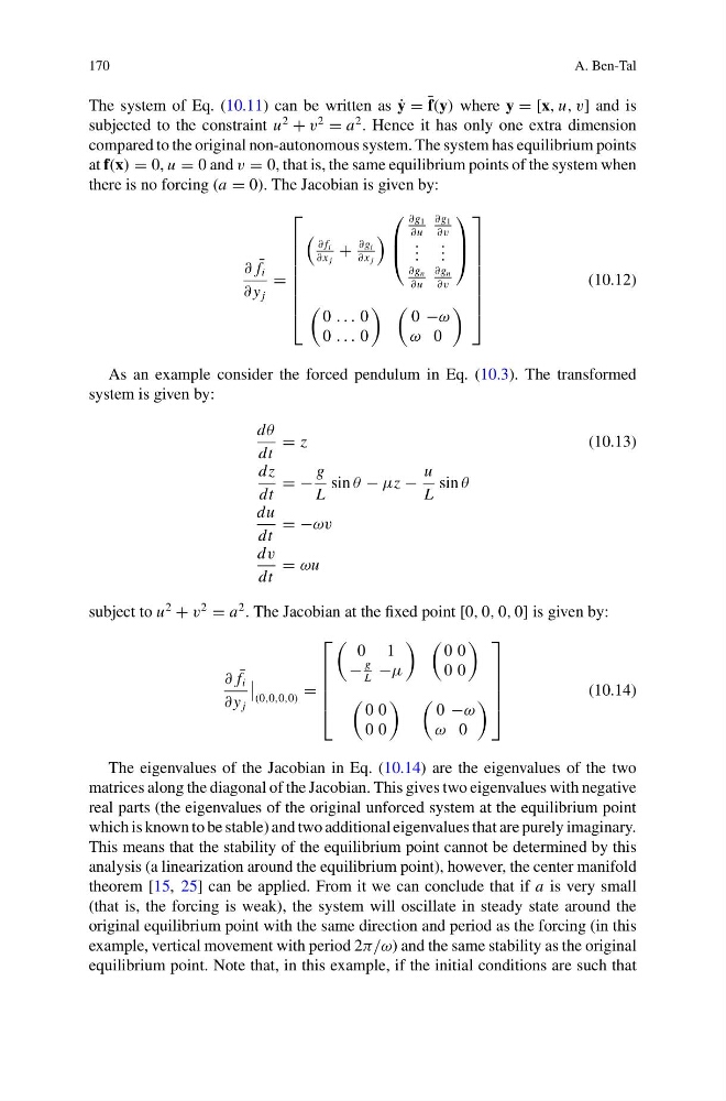
The eigenvalues of the Jacobian in Eq. (10.14) are the eigenvalues of the two
matrices along the diagonal of the Jacobian. This gives two eigenvalues with negative
real parts (the eigenvalues of the original unforced system at the equilibrium point
which is known to be stable) and two additional eigenvalues that are purely imaginary.
This means that the stability of the equilibrium point cannot be determined by this
analysis (a linearization around the equilibrium point), however, the center manifold
theorem [15, 25] can be applied. From it we can conclude that if a is very small
(that is, the forcing is weak), the system will oscillate in steady state around the
original equilibrium point with the same direction and period as the forcing (in this
example, vertical movement with period 2π/ω) and the same stability as the original
equilibrium point. Note that, in this example, if the initial conditions are such that
A. Ben-Tal
The system of Eq. (10.11) can be written as ˙
y = ¯ f(y) where y = [x, u, v] and is
subjected to the constraint u
2
+ v
2
= a
2 . Hence it has only one extra dimension
compared to the original non-autonomous system. The system has equilibrium points
at f(x) = 0, u = 0 and v = 0, that is, the same equilibrium points of the system when
there is no forcing (a = 0). The Jacobian is given by:
∂ ¯
f i
∂ y j
=
⎡
⎢
⎢
⎢
⎢
⎢
⎢
⎢
⎣
∂ f i
∂ x j
+
∂g i
∂ x j
⎛
⎜
⎝
∂g 1
∂u
∂g 1
∂v
. . .
. . .
∂g n
∂u
∂g n
∂v
⎞
⎟
⎠
0 . . . 0
0 . . . 0
0 −ω
ω 0
⎤
⎥
⎥
⎥
⎥
⎥
⎥
⎥
⎦
(10.12)
As an example consider the forced pendulum in Eq. (10.3). The transformed
system is given by:
dθ
dt
= z
(10.13)
dz
dt
= −
g
L
sin θ − μz −
u
L
sin θ
du
dt
= −ωv
dv
dt
= ωu
subject to u
2
+ v
2
= a
2 . The Jacobian at the fixed point [0, 0, 0, 0] is given by:
∂ ¯
f i
∂ y j
(0,0,0,0)
=
⎡
⎢
⎢
⎢
⎢
⎣
0 1
−
g
L
−μ
0 0
0 0
0 0
0 0
0 −ω
ω 0
⎤
⎥
⎥
⎥
⎥
⎦
(10.14)
The eigenvalues of the Jacobian in Eq. (10.14) are the eigenvalues of the two
matrices along the diagonal of the Jacobian. This gives two eigenvalues with negative
real parts (the eigenvalues of the original unforced system at the equilibrium point
which is known to be stable) and two additional eigenvalues that are purely imaginary.
This means that the stability of the equilibrium point cannot be determined by this
analysis (a linearization around the equilibrium point), however, the center manifold
theorem [15, 25] can be applied. From it we can conclude that if a is very small
(that is, the forcing is weak), the system will oscillate in steady state around the
original equilibrium point with the same direction and period as the forcing (in this
example, vertical movement with period 2π/ω) and the same stability as the original
equilibrium point. Note that, in this example, if the initial conditions are such that