

9 On Localised Modes in Bio-inspired Hierarchically Organised …
157
two pairs of block masses m 2 are attached to two masses m 1 by parallel linear springs
of equal stiffness k 2 .
Following the algorithm from the previous section, it is assumed that the reduction
of the parameters follows the laws:
m 1
m
=
m 2
m 1
=
1
2
4
3 ,
k 1
k
=
k 2
k 1
= κ [3]. Four absolute
generalised coordinates z 1 –z 4 are introduced (Fig. 9.4). Deriving the equations of
motion as in Sect. 9.2, assuming the harmonic solutions for each coordinate, the
following corresponding characteristic equation [7] can be obtained:
22 = 22,1 22,2 22,3 = 0,
(9.7)
where:
22,1 =
k 2 − m 2 ω
2
2 ,
(9.8)
22,2 = k 1 k 2 − (k 2 m 1 + k 1 m 2 + 2k 2 m 2 )ω
2
+ m 1 m 2 ω
4
,
(9.9)
22,3 = kk 1 k 2 − (k 1 k 2 m + kk 2 m 1 +2k 1 k 2 m 1 + kk 1 m 2 +2kk 2 m 2 +4k 1 k 2 m 2 )ω
2
+ (k 2 mm 1 + k 1 mm 2 +2k 2 mm 2 + km 1 m 2 +2k 1 m 1 m 2 )ω
4
− mm 1 m 2 ω
6
,
(9.10)
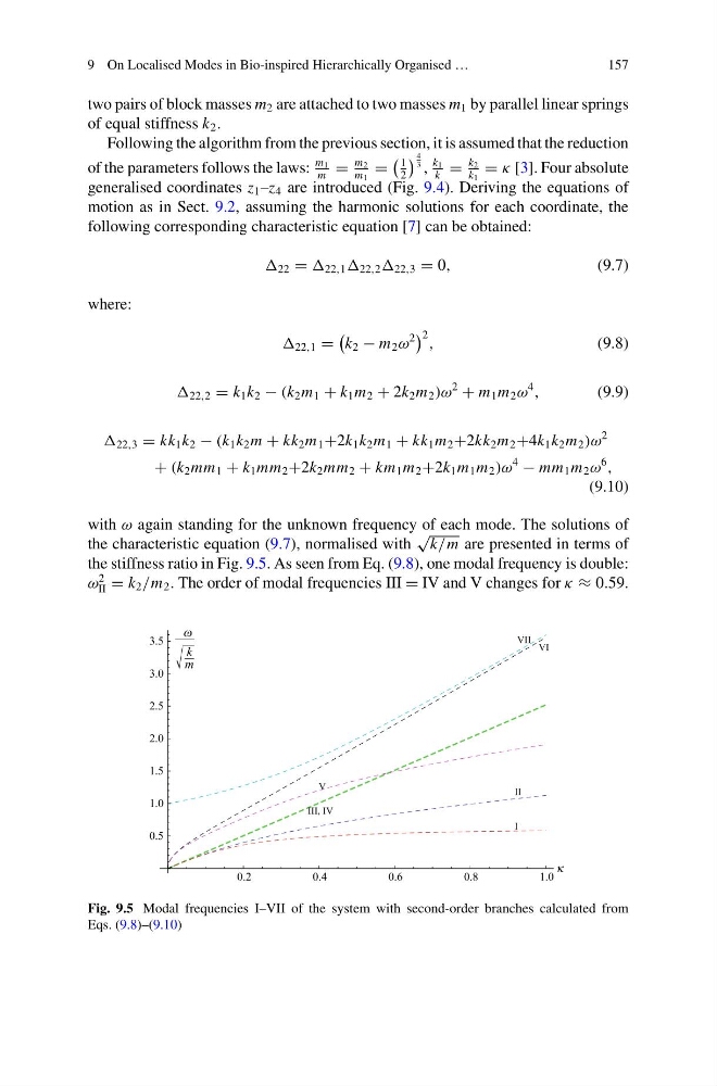
with ω again standing for the unknown frequency of each mode. The solutions of
the characteristic equation (9.7), normalised with
√
k/m are presented in terms of
the stiffness ratio in Fig. 9.5. As seen from Eq. (9.8), one modal frequency is double:
ω
2
II = k 2 /m 2 . The order of modal frequencies III = IV and V changes for κ ≈ 0.59.
0.2
0.4
0.6
0.8
1.0
0.5
1.0
1.5
2.0
2.5
3.0
3.5
I
II
III, IV
VI
VII
V
k
m
Fig. 9.5 Modal frequencies I–VII of the system with second-order branches calculated from
Eqs. (9.8)–(9.10)
157
two pairs of block masses m 2 are attached to two masses m 1 by parallel linear springs
of equal stiffness k 2 .
Following the algorithm from the previous section, it is assumed that the reduction
of the parameters follows the laws:
m 1
m
=
m 2
m 1
=
1
2
4
3 ,
k 1
k
=
k 2
k 1
= κ [3]. Four absolute
generalised coordinates z 1 –z 4 are introduced (Fig. 9.4). Deriving the equations of
motion as in Sect. 9.2, assuming the harmonic solutions for each coordinate, the
following corresponding characteristic equation [7] can be obtained:
22 = 22,1 22,2 22,3 = 0,
(9.7)
where:
22,1 =
k 2 − m 2 ω
2
2 ,
(9.8)
22,2 = k 1 k 2 − (k 2 m 1 + k 1 m 2 + 2k 2 m 2 )ω
2
+ m 1 m 2 ω
4
,
(9.9)
22,3 = kk 1 k 2 − (k 1 k 2 m + kk 2 m 1 +2k 1 k 2 m 1 + kk 1 m 2 +2kk 2 m 2 +4k 1 k 2 m 2 )ω
2
+ (k 2 mm 1 + k 1 mm 2 +2k 2 mm 2 + km 1 m 2 +2k 1 m 1 m 2 )ω
4
− mm 1 m 2 ω
6
,
(9.10)
with ω again standing for the unknown frequency of each mode. The solutions of
the characteristic equation (9.7), normalised with
√
k/m are presented in terms of
the stiffness ratio in Fig. 9.5. As seen from Eq. (9.8), one modal frequency is double:
ω
2
II = k 2 /m 2 . The order of modal frequencies III = IV and V changes for κ ≈ 0.59.
0.2
0.4
0.6
0.8
1.0
0.5
1.0
1.5
2.0
2.5
3.0
3.5
I
II
III, IV
VI
VII
V
k
m
Fig. 9.5 Modal frequencies I–VII of the system with second-order branches calculated from
Eqs. (9.8)–(9.10)