

9 On Localised Modes in Bio-inspired Hierarchically Organised …
155
21 =
k + 2k 1 − mω
2
−k 1
−k 1
−k 1
k 1 − m 1 ω
2
0
−k 1
0
k 1 − m 1 ω
2
= 0.
(9.4)
This equation can be represented as 21 = 21,1 21,2 = 0, where
21,1 =
k 1 − m 1 ω
2
,
(9.5)
21,2 =
kk 1 − (k 1 m + km 1 + 2k 1 m 1 )ω
2
+ mm 1 ω
4
= 0.
(9.6)
Based on previous experiments that the masses and stiffness reduce with a new
order of hierarchy, the corresponding reduction laws are taken as follows:
m 1
m
=
1
2
4
3 ,
k 1
k
= κ (see [3] and the references cited there). The parameter κ represent the stiffness
ratio.
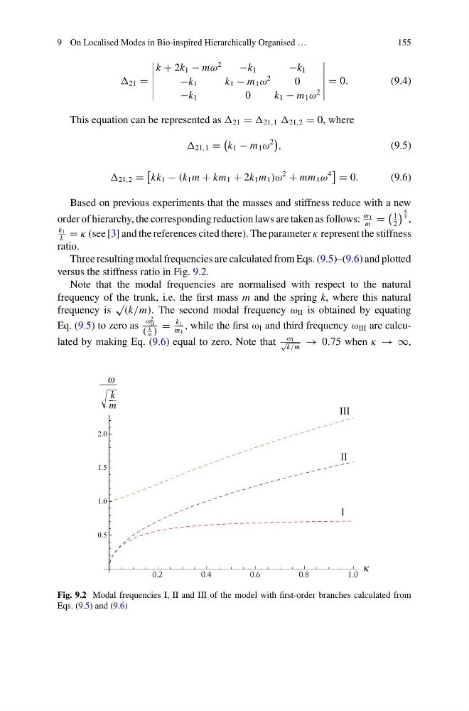
Three resulting modal frequencies are calculated from Eqs. (9.5)–(9.6) and plotted
versus the stiffness ratio in Fig. 9.2.
Note that the modal frequencies are normalised with respect to the natural
frequency of the trunk, i.e. the first mass m and the spring k, where this natural
frequency is
√
(k/m). The second modal frequency ω II is obtained by equating
Eq. (9.5) to zero as
ω
2
II
(
k
m )
=
k 1
m 1
, while the first ω I and third frequency ω III are calculated by making Eq. (9.6) equal to zero. Note that
ω I
√
k/m
→ 0.75 when κ → ∞,
0.2
0.4
0.6
0.8
1.0
0.5
1.0
1.5
2.0
k
m
III
II
I
Fig. 9.2 Modal frequencies I, II and III of the model with first-order branches calculated from
Eqs. (9.5) and (9.6)
155
21 =
k + 2k 1 − mω
2
−k 1
−k 1
−k 1
k 1 − m 1 ω
2
0
−k 1
0
k 1 − m 1 ω
2
= 0.
(9.4)
This equation can be represented as 21 = 21,1 21,2 = 0, where
21,1 =
k 1 − m 1 ω
2
,
(9.5)
21,2 =
kk 1 − (k 1 m + km 1 + 2k 1 m 1 )ω
2
+ mm 1 ω
4
= 0.
(9.6)
Based on previous experiments that the masses and stiffness reduce with a new
order of hierarchy, the corresponding reduction laws are taken as follows:
m 1
m
=
1
2
4
3 ,
k 1
k
= κ (see [3] and the references cited there). The parameter κ represent the stiffness
ratio.
Three resulting modal frequencies are calculated from Eqs. (9.5)–(9.6) and plotted
versus the stiffness ratio in Fig. 9.2.
Note that the modal frequencies are normalised with respect to the natural
frequency of the trunk, i.e. the first mass m and the spring k, where this natural
frequency is
√
(k/m). The second modal frequency ω II is obtained by equating
Eq. (9.5) to zero as
ω
2
II
(
k
m )
=
k 1
m 1
, while the first ω I and third frequency ω III are calculated by making Eq. (9.6) equal to zero. Note that
ω I
√
k/m
→ 0.75 when κ → ∞,
0.2
0.4
0.6
0.8
1.0
0.5
1.0
1.5
2.0
k
m
III
II
I
Fig. 9.2 Modal frequencies I, II and III of the model with first-order branches calculated from
Eqs. (9.5) and (9.6)