

106
M. Lucas et al.
6.4.5 Network: Time-Varying Driving Strength
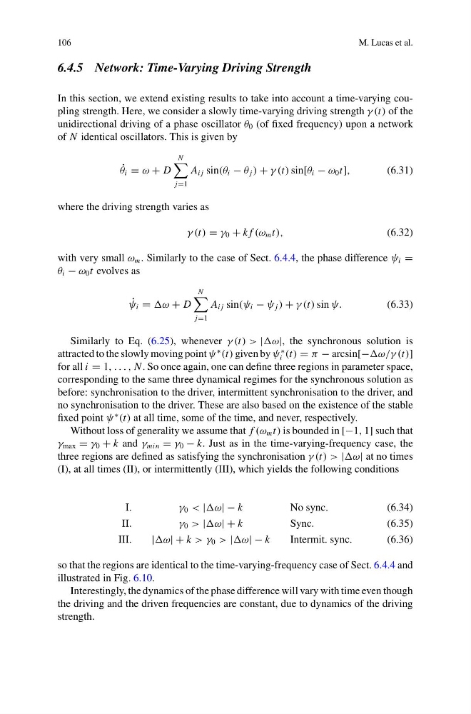
In this section, we extend existing results to take into account a time-varying coupling strength. Here, we consider a slowly time-varying driving strength γ (t) of the
unidirectional driving of a phase oscillator θ 0 (of fixed frequency) upon a network
of N identical oscillators. This is given by
˙
θ i = ω + D
N
j=1
A i j sin(θ i − θ j ) + γ (t) sin[θ i − ω 0 t],
(6.31)
where the driving strength varies as
γ (t) = γ 0 + k f (ω m t),
(6.32)
with very small ω m . Similarly to the case of Sect. 6.4.4, the phase difference ψ i =
θ i − ω 0 t evolves as
˙
ψ i = ω + D
N
j=1
A i j sin(ψ i − ψ j ) + γ (t) sin ψ.
(6.33)
Similarly to Eq. (6.25), whenever γ (t) > |ω|, the synchronous solution is
attracted to the slowly moving point ψ
∗
(t) given by ψ
∗
i (t) = π − arcsin[− (t)]
for all i = 1, . . . , N . So once again, one can define three regions in parameter space,
corresponding to the same three dynamical regimes for the synchronous solution as
before: synchronisation to the driver, intermittent synchronisation to the driver, and
no synchronisation to the driver. These are also based on the existence of the stable
fixed point ψ
∗
(t) at all time, some of the time, and never, respectively.
Without loss of generality we assume that f (ω m t) is bounded in [−1, 1] such that
γ max = γ 0 + k and γ min = γ 0 − k. Just as in the time-varying-frequency case, the
three regions are defined as satisfying the synchronisation γ (t) > |ω| at no times
(I), at all times (II), or intermittently (III), which yields the following conditions
I.
γ 0 < |ω| − k
No sync.
(6.34)
II.
γ 0 > |ω| + k
Sync.
(6.35)
III.
|ω| + k > γ 0 > |ω| − k
Intermit. sync.
(6.36)
so that the regions are identical to the time-varying-frequency case of Sect. 6.4.4 and
illustrated in Fig. 6.10.
Interestingly, the dynamics of the phase difference will vary with time even though
the driving and the driven frequencies are constant, due to dynamics of the driving
strength.
M. Lucas et al.
6.4.5 Network: Time-Varying Driving Strength
In this section, we extend existing results to take into account a time-varying coupling strength. Here, we consider a slowly time-varying driving strength γ (t) of the
unidirectional driving of a phase oscillator θ 0 (of fixed frequency) upon a network
of N identical oscillators. This is given by
˙
θ i = ω + D
N
j=1
A i j sin(θ i − θ j ) + γ (t) sin[θ i − ω 0 t],
(6.31)
where the driving strength varies as
γ (t) = γ 0 + k f (ω m t),
(6.32)
with very small ω m . Similarly to the case of Sect. 6.4.4, the phase difference ψ i =
θ i − ω 0 t evolves as
˙
ψ i = ω + D
N
j=1
A i j sin(ψ i − ψ j ) + γ (t) sin ψ.
(6.33)
Similarly to Eq. (6.25), whenever γ (t) > |ω|, the synchronous solution is
attracted to the slowly moving point ψ
∗
(t) given by ψ
∗
i (t) = π − arcsin[− (t)]
for all i = 1, . . . , N . So once again, one can define three regions in parameter space,
corresponding to the same three dynamical regimes for the synchronous solution as
before: synchronisation to the driver, intermittent synchronisation to the driver, and
no synchronisation to the driver. These are also based on the existence of the stable
fixed point ψ
∗
(t) at all time, some of the time, and never, respectively.
Without loss of generality we assume that f (ω m t) is bounded in [−1, 1] such that
γ max = γ 0 + k and γ min = γ 0 − k. Just as in the time-varying-frequency case, the
three regions are defined as satisfying the synchronisation γ (t) > |ω| at no times
(I), at all times (II), or intermittently (III), which yields the following conditions
I.
γ 0 < |ω| − k
No sync.
(6.34)
II.
γ 0 > |ω| + k
Sync.
(6.35)
III.
|ω| + k > γ 0 > |ω| − k
Intermit. sync.
(6.36)
so that the regions are identical to the time-varying-frequency case of Sect. 6.4.4 and
illustrated in Fig. 6.10.
Interestingly, the dynamics of the phase difference will vary with time even though
the driving and the driven frequencies are constant, due to dynamics of the driving
strength.