

6 Synchronisation and Non-autonomicity
105
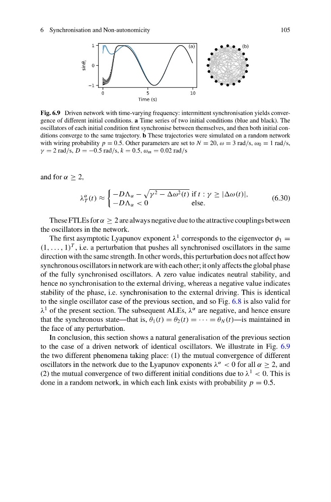
Fig. 6.9 Driven network with time-varying frequency: intermittent synchronisation yields convergence of different initial conditions. a Time series of two initial conditions (blue and black). The
oscillators of each initial condition first synchronise between themselves, and then both initial conditions converge to the same trajectory. b These trajectories were simulated on a random network
with wiring probability p = 0.5. Other parameters are set to N = 20, ω = 3 rad/s, ω 0 = 1 rad/s,
γ = 2 rad/s, D = −0.5 rad/s, k = 0.5, ω m = 0.02 rad/s
and for α ≥ 2,
λ
α
T (t) ≈
−D α −
γ 2 − 2 (t) if t : γ ≥ |ω(t)|,
−D α < 0
e l s e .
(6.30)
These FTLEs for α ≥ 2 are always negative due to the attractive couplings between
the oscillators in the network.
The first asymptotic Lyapunov exponent λ
1 corresponds to the eigenvector φ 1 =
(1, . . . , 1)
T , i.e. a perturbation that pushes all synchronised oscillators in the same
direction with the same strength. In other words, this perturbation does not affect how
synchronous oscillators in network are with each other; it only affects the global phase
of the fully synchronised oscillators. A zero value indicates neutral stability, and
hence no synchronisation to the external driving, whereas a negative value indicates
stability of the phase, i.e. synchronisation to the external driving. This is identical
to the single oscillator case of the previous section, and so Fig. 6.8 is also valid for
λ
1 of the present section. The subsequent ALEs, λ
α are negative, and hence ensure
that the synchronous state—that is, θ 1 (t) = θ 2 (t) = · · · = θ N (t)—is maintained in
the face of any perturbation.
In conclusion, this section shows a natural generalisation of the previous section
to the case of a driven network of identical oscillators. We illustrate in Fig. 6.9
the two different phenomena taking place: (1) the mutual convergence of different
oscillators in the network due to the Lyapunov exponents λ
α
< 0 for all α ≥ 2, and
(2) the mutual convergence of two different initial conditions due to λ
1
< 0. This is
done in a random network, in which each link exists with probability p = 0.5.
105
Fig. 6.9 Driven network with time-varying frequency: intermittent synchronisation yields convergence of different initial conditions. a Time series of two initial conditions (blue and black). The
oscillators of each initial condition first synchronise between themselves, and then both initial conditions converge to the same trajectory. b These trajectories were simulated on a random network
with wiring probability p = 0.5. Other parameters are set to N = 20, ω = 3 rad/s, ω 0 = 1 rad/s,
γ = 2 rad/s, D = −0.5 rad/s, k = 0.5, ω m = 0.02 rad/s
and for α ≥ 2,
λ
α
T (t) ≈
−D α −
γ 2 − 2 (t) if t : γ ≥ |ω(t)|,
−D α < 0
e l s e .
(6.30)
These FTLEs for α ≥ 2 are always negative due to the attractive couplings between
the oscillators in the network.
The first asymptotic Lyapunov exponent λ
1 corresponds to the eigenvector φ 1 =
(1, . . . , 1)
T , i.e. a perturbation that pushes all synchronised oscillators in the same
direction with the same strength. In other words, this perturbation does not affect how
synchronous oscillators in network are with each other; it only affects the global phase
of the fully synchronised oscillators. A zero value indicates neutral stability, and
hence no synchronisation to the external driving, whereas a negative value indicates
stability of the phase, i.e. synchronisation to the external driving. This is identical
to the single oscillator case of the previous section, and so Fig. 6.8 is also valid for
λ
1 of the present section. The subsequent ALEs, λ
α are negative, and hence ensure
that the synchronous state—that is, θ 1 (t) = θ 2 (t) = · · · = θ N (t)—is maintained in
the face of any perturbation.
In conclusion, this section shows a natural generalisation of the previous section
to the case of a driven network of identical oscillators. We illustrate in Fig. 6.9
the two different phenomena taking place: (1) the mutual convergence of different
oscillators in the network due to the Lyapunov exponents λ
α
< 0 for all α ≥ 2, and
(2) the mutual convergence of two different initial conditions due to λ
1
< 0. This is
done in a random network, in which each link exists with probability p = 0.5.