

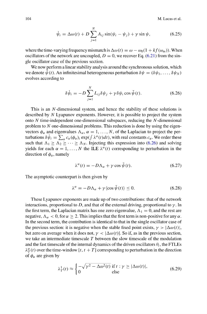
104
M. Lucas et al.
˙
ψ i = ω(t) + D
N
j=1
A i j sin(ψ i − ψ j ) + γ sin ψ,
(6.25)
where the time-varying frequency mismatch is ω(t) = ω − ω 0 (1 + k f (ω m )). When
oscillators of the network are uncoupled, D = 0, we recover Eq. (6.21) from the single oscillator case of the previous section.
We now perform a linear stability analysis around the synchronous solution, which
we denote ˜
ψ(t). An infinitesimal heterogeneous perturbation δψ = (δψ 1 , . . . , δψ N )
evolves according to
δ ˙
ψ i = −D
N
j=1
L i j δψ j + γ δψ i cos ˜
ψ(t).
(6.26)
This is an N -dimensional system, and hence the stability of these solutions is
described by N Lyapunov exponents. However, it is possible to project the system
onto N time-independent one-dimensional subspaces, reducing the N -dimensional
problem to N one-dimensional problems. This reduction is done by using the eigenvectors φ α and eigenvalues α , α = 1, . . . , N , of the Laplacian to project the perturbations δ ˙
ψ i =
α c α (φ α ) i exp(
λ
α
(t)dt), with real constants c α . We order these
such that 1 ≥ 2 ≥ · · · ≥ N . Injecting this expression into (6.26) and solving
yields for each α = 1, . . . , N the ILE λ
α
(t) corresponding to perturbation in the
direction of φ α , namely
λ
α
(t) = −D α + γ cos ˜
ψ(t).
(6.27)
The asymptotic counterpart is then given by
λ
α
= −D α + γ cos ˜
ψ(t) ≤ 0.
(6.28)
These Lyapunov exponents are made up of two contributions: that of the network
interactions, proportional to D, and that of the external driving, proportional to γ . In
the first term, the Laplacian matrix has one zero eigenvalue, 1 = 0, and the rest are
negative, α < 0, for α ≥ 2. This implies that the first term is non-positive for any α.
In the second term, the contribution is identical to that in the single oscillator case of
the previous section: it is negative when the stable fixed point exists, γ > |
but zero on average when it does not, γ < | So if, as in the previous section,
we take an intermediate timescale T between the slow timescale of the modulation
and the fast timescale of the internal dynamics of the driven oscillators θ i , the FTLEs
λ
α
T (t) over the time-window [t, t + T ] corresponding to perturbation in the direction
of φ α are given by
λ
1
T (t) ≈
−
γ 2 − ω 2 (t) if t : γ ≥ |ω(t)|,
0
e l s e
(6.29)
M. Lucas et al.
˙
ψ i = ω(t) + D
N
j=1
A i j sin(ψ i − ψ j ) + γ sin ψ,
(6.25)
where the time-varying frequency mismatch is ω(t) = ω − ω 0 (1 + k f (ω m )). When
oscillators of the network are uncoupled, D = 0, we recover Eq. (6.21) from the single oscillator case of the previous section.
We now perform a linear stability analysis around the synchronous solution, which
we denote ˜
ψ(t). An infinitesimal heterogeneous perturbation δψ = (δψ 1 , . . . , δψ N )
evolves according to
δ ˙
ψ i = −D
N
j=1
L i j δψ j + γ δψ i cos ˜
ψ(t).
(6.26)
This is an N -dimensional system, and hence the stability of these solutions is
described by N Lyapunov exponents. However, it is possible to project the system
onto N time-independent one-dimensional subspaces, reducing the N -dimensional
problem to N one-dimensional problems. This reduction is done by using the eigenvectors φ α and eigenvalues α , α = 1, . . . , N , of the Laplacian to project the perturbations δ ˙
ψ i =
α c α (φ α ) i exp(
λ
α
(t)dt), with real constants c α . We order these
such that 1 ≥ 2 ≥ · · · ≥ N . Injecting this expression into (6.26) and solving
yields for each α = 1, . . . , N the ILE λ
α
(t) corresponding to perturbation in the
direction of φ α , namely
λ
α
(t) = −D α + γ cos ˜
ψ(t).
(6.27)
The asymptotic counterpart is then given by
λ
α
= −D α + γ cos ˜
ψ(t) ≤ 0.
(6.28)
These Lyapunov exponents are made up of two contributions: that of the network
interactions, proportional to D, and that of the external driving, proportional to γ . In
the first term, the Laplacian matrix has one zero eigenvalue, 1 = 0, and the rest are
negative, α < 0, for α ≥ 2. This implies that the first term is non-positive for any α.
In the second term, the contribution is identical to that in the single oscillator case of
the previous section: it is negative when the stable fixed point exists, γ > |
but zero on average when it does not, γ < | So if, as in the previous section,
we take an intermediate timescale T between the slow timescale of the modulation
and the fast timescale of the internal dynamics of the driven oscillators θ i , the FTLEs
λ
α
T (t) over the time-window [t, t + T ] corresponding to perturbation in the direction
of φ α are given by
λ
1
T (t) ≈
−
γ 2 − ω 2 (t) if t : γ ≥ |ω(t)|,
0
e l s e
(6.29)