

6 Synchronisation and Non-autonomicity
101
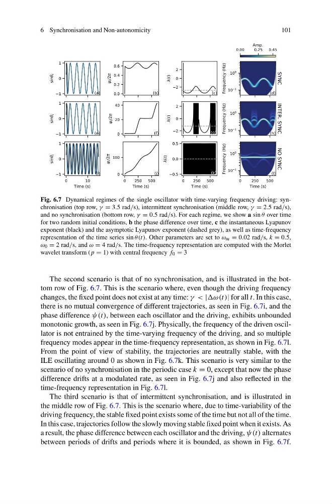
Fig. 6.7 Dynamical regimes of the single oscillator with time-varying frequency driving: synchronisation (top row, γ = 3.5 rad/s), intermittent synchronisation (middle row, γ = 2.5 rad/s),
and no synchronisation (bottom row, γ = 0.5 rad/s). For each regime, we show a sin θ over time
for two random initial conditions, b the phase difference over time, c the instantaneous Lyapunov
exponent (black) and the asymptotic Lyapunov exponent (dashed grey), as well as time-frequency
representation of the time series sin θ(t). Other parameters are set to ω m = 0.02 rad/s, k = 0.5,
ω 0 = 2 rad/s, and ω = 4 rad/s. The time-frequency representation are computed with the Morlet
wavelet transform ( p = 1) with central frequency f 0 = 3
The second scenario is that of no synchronisation, and is illustrated in the bottom row of Fig. 6.7. This is the scenario where, even though the driving frequency
changes, the fixed point does not exist at any time: γ < | for all t. In this case,
there is no mutual convergence of different trajectories, as seen in Fig. 6.7i, and the
phase difference ψ(t), between each oscillator and the driving, exhibits unbounded
monotonic growth, as seen in Fig. 6.7j. Physically, the frequency of the driven oscillator is not entrained by the time-varying frequency of the driving, and so multiple
frequency modes appear in the time-frequency representation, as shown in Fig. 6.7l.
From the point of view of stability, the trajectories are neutrally stable, with the
ILE oscillating around 0 as shown in Fig. 6.7k. This scenario is very similar to the
scenario of no synchronisation in the periodic case k = 0, except that now the phase
difference drifts at a modulated rate, as seen in Fig. 6.7j and also reflected in the
time-frequency representation in Fig. 6.7l.
The third scenario is that of intermittent synchronisation, and is illustrated in
the middle row of Fig. 6.7. This is the scenario where, due to time-variability of the
driving frequency, the stable fixed point exists some of the time but not all of the time.
In this case, trajectories follow the slowly moving stable fixed point when it exists. As
a result, the phase difference between each oscillator and the driving, ψ(t) alternates
between periods of drifts and periods where it is bounded, as shown in Fig. 6.7f.
101
Fig. 6.7 Dynamical regimes of the single oscillator with time-varying frequency driving: synchronisation (top row, γ = 3.5 rad/s), intermittent synchronisation (middle row, γ = 2.5 rad/s),
and no synchronisation (bottom row, γ = 0.5 rad/s). For each regime, we show a sin θ over time
for two random initial conditions, b the phase difference over time, c the instantaneous Lyapunov
exponent (black) and the asymptotic Lyapunov exponent (dashed grey), as well as time-frequency
representation of the time series sin θ(t). Other parameters are set to ω m = 0.02 rad/s, k = 0.5,
ω 0 = 2 rad/s, and ω = 4 rad/s. The time-frequency representation are computed with the Morlet
wavelet transform ( p = 1) with central frequency f 0 = 3
The second scenario is that of no synchronisation, and is illustrated in the bottom row of Fig. 6.7. This is the scenario where, even though the driving frequency
changes, the fixed point does not exist at any time: γ < | for all t. In this case,
there is no mutual convergence of different trajectories, as seen in Fig. 6.7i, and the
phase difference ψ(t), between each oscillator and the driving, exhibits unbounded
monotonic growth, as seen in Fig. 6.7j. Physically, the frequency of the driven oscillator is not entrained by the time-varying frequency of the driving, and so multiple
frequency modes appear in the time-frequency representation, as shown in Fig. 6.7l.
From the point of view of stability, the trajectories are neutrally stable, with the
ILE oscillating around 0 as shown in Fig. 6.7k. This scenario is very similar to the
scenario of no synchronisation in the periodic case k = 0, except that now the phase
difference drifts at a modulated rate, as seen in Fig. 6.7j and also reflected in the
time-frequency representation in Fig. 6.7l.
The third scenario is that of intermittent synchronisation, and is illustrated in
the middle row of Fig. 6.7. This is the scenario where, due to time-variability of the
driving frequency, the stable fixed point exists some of the time but not all of the time.
In this case, trajectories follow the slowly moving stable fixed point when it exists. As
a result, the phase difference between each oscillator and the driving, ψ(t) alternates
between periods of drifts and periods where it is bounded, as shown in Fig. 6.7f.